4. Calculating Coulomb interactions and the charge stability diagram of a quantum dot
4.1. Requirements
4.1.1. Software components
QTCAD®
4.1.2. Mesh file
qtcad/examples/practical_application/Ge_hole/meshes/refined_gedqd.msh
4.1.3. Python script
qtcad/examples/practical_application/Ge_hole/4-CSD.py
4.1.4. References
4.2. Briefing
In this tutorial, we build on the previously computed lever-arm matrix and single-particle quantum dot spectrum to study many-body effects in a Ge-based double quantum dot system.
Hole transport in such devices is governed by Coulomb interactions between holes. These interactions make the energy required to add a carrier depend on the dot occupation, giving rise to Coulomb blockade. In this regime, transport is suppressed except when two many-body charge states with different integer particle numbers become degenerate. These degeneracy conditions define the boundaries of the Coulomb blockade regions and form the characteristic Coulomb diamonds observed in the stability diagram.
To capture this physics, we:
Solve the single-particle Schrödinger problem in the dot region;
Construct and diagonalize the interacting many-body Hamiltonian;
Use the previously computed lever-arm matrix to map gate voltages to transport observables;
Evaluate the charge stability diagram via a transport response function.
The final result is a two-dimensional stability map showing how transport depends on multiple gate voltages.
4.3. Setting up the device
4.3.1. Header
We begin by importing the required QTCAD modules for quantum transport, many-body physics, and device analysis.
from qtcad.device import materials as mt
from qtcad.device import io
from qtcad.device.mesh3d import Mesh, SubMesh
from qtcad.device import Device, SubDevice
from qtcad.device.many_body import Solver as ManyBodySolver
from qtcad.device.many_body import SolverParams as ManyBodySolverParams
from qtcad.device.schrodinger import Solver as SchrodingerSolver
from qtcad.device.schrodinger import SolverParams as SchrodingerSolverParams
from qtcad.transport.junction import Junction
from qtcad.transport.mastereq import add_spectrum
import numpy as np
from pathlib import Path
from matplotlib import pyplot as plt
These modules provide the full workflow, including single-particle Schrödinger eigenstate calculations, many-body solvers, and transport calculations for obtaining the charge stability diagram.
4.4. Defining paths and loading the mesh
We define the simulation paths and the location of the refined double quantum dot mesh introduced in the Simulating hole states in a Ge/SiGe quantum dot using Poisson and Schrödinger solvers tutorial.
script_dir = Path(__file__).parent.resolve()
mesh_dir = script_dir / "meshes"
mesh_file_dir = mesh_dir / "refined_gedqd.msh"
xao_dir = mesh_dir / "ge_dqd.xao"
out_dir = script_dir / "output"
out_dir.mkdir(exist_ok=True)
The mesh is then loaded with nanometer scaling:
scaling = 1e-9  # nanometers
mesh = Mesh(scaling, mesh_file_dir)
4.5. Device construction and quantum dot definition
We load the mesh, define the Ge/SiGe heterostructure, and construct the quantum dot region as in the previous tutorials (Simulating bound states in a quantum dot using the Poisson and Schrödinger solvers).
dvc = Device(mesh, conf_carriers='h', hole_kp_model="luttinger_kohn_foreman")
dvc.set_temperature(0.1)
As shown in Simulating bound states in a quantum dot using the Poisson and Schrödinger solvers tutorial, we assign a material to each specified region.
# Assign the material to regions
dvc.new_region("substrate", mt.SiGe_DFT)
dvc.new_region("SiGe_barrier", mt.SiGe_DFT)
dvc.new_region("Ge_well", mt.Ge)
dvc.new_region("SiGe_cap", mt.SiGe_DFT)
dvc.new_region("oxide", mt.Al2O3)

# Dot-region volumes
dvc.new_region("Ge_well.dot_region", mt.Ge)
dvc.new_region("SiGe_barrier.dot_region", mt.SiGe_DFT)
dvc.new_region("SiGe_cap.dot_region", mt.SiGe_DFT)
4.6. Boundary conditions
Gate electrodes are defined using fixed bias voltages applied at selected boundaries. These gates control confinement and are the parameters varied in the lever-arm analysis.
# boundary conditions
Ew = mt.Ge.chi + 1.1*mt.Ge.Eg
dvc.new_gate_bnd("P1", -0.6, Ew)
dvc.new_gate_bnd("P2", -0.6, Ew)
dvc.new_gate_bnd("BC", 0.9, Ew)
dvc.new_gate_bnd("BL", 0.5, Ew)
dvc.new_gate_bnd("BR", 0.5, Ew)

dot_region_list = [
    "Ge_well.dot_region",
    "SiGe_barrier.dot_region",
    "SiGe_cap.dot_region"
]

dvc.set_dot_region(dot_region_list)
The electrostatic confinement potential is imported from the previous tutorial.
phi = io.load(out_dir / 'electrostatic_potential.hdf5')
dvc.set_potential(phi)

dvc.set_V_from_phi()
A subdevice is then created to restrict Schrödinger and many-body calculations to the dot region only:
submesh = SubMesh(dvc.mesh, dot_region_list)
subdvc = SubDevice(dvc, submesh)
4.7. Solving the single-particle problem
We first compute the single-particle eigenstates, which form the basis for the many-body Hamiltonian.
schrodinger_params = SchrodingerSolverParams()
schrodinger_params.num_states = 20
schrodinger_params.tol = 1e-5

schrodinger_solver = SchrodingerSolver(subdvc, solver_params=schrodinger_params)
schrodinger_solver.solve()
The resulting eigenenergies define the orbital basis used for Coulomb interaction calculations.
We then inspect the spectrum:
subdvc.print_energies()
energies = subdvc.energies
4.8. Many-body Hamiltonian and Coulomb interactions
We construct the many-body Solver
which computes Coulomb integrals between confined states and builds the many-body Hamiltonian.
many_body_solver_params = ManyBodySolverParams()
many_body_solver_params.n_degen = 1
many_body_solver_params.num_states = 8

slv = ManyBodySolver(subdvc, solver_params=many_body_solver_params)
Since the single-particle hole states already include the spin degree
of freedom, we set the many-body solver parameter n_degen to 1.
In contrast, in electron-based examples this parameter is typically set to 2,
because the single-particle states do not explicitly account for spin.
After diagonalization, the solver provides:
Coulomb integrals
chemical potentials,
Coulomb peak positions,
and the interacting energy spectrum.
We extract Coulomb interaction terms explicitly:
coulomb_overlap = slv.get_coulomb_matrix(overlap=True, verbose=True)
np.save(out_dir / "coulomb_mat_overlap.npy", coulomb_overlap)
4.9. Transport model and junction construction
To model transport, we construct a Junction
that couples the quantum dots to leads. While such leads can in principle be modeled explicitly
within QTCAD, in this example they are not represented as physical structures.
Instead, they are treated as effective reservoirs that enable the description
of charge transport. The previously computed lever-arm matrix is used to convert
gate voltages into energy shifts. For more details, see Transport in the Coulomb blockade regime.
temperature_spec = 10  # Kelvin

lever_arm_matrix = np.load(out_dir / "lever_arm_matrix.npy")

gate_labels = ["BL", "P1", "P2", "BR"]

many_body_solver_params.energies = energies
many_body_solver_params.overlap = True
many_body_solver_params.coulomb_mat = coulomb_overlap
many_body_solver_params.alpha = lever_arm_matrix

jc = Junction(
    many_body_solver_params=many_body_solver_params,
    temperature=temperature_spec,
    contact_labels=gate_labels
)
The junction enables evaluation of transport observables via rate equations.
In this simulation, we increase the junction temperature to \(10\ \mathrm{K}\). This is done to broaden the transition lines, which makes the charge stability diagram easier to resolve while reducing the computational cost.
4.10. Charge stability diagram computation
We compute the particle addition spectrum by calling the
add_spectrum method of the
mastereq module over a two-dimensional
sweep of gate voltages. This quantity captures the transport response
of the quantum-dot system. In the regime of small source-drain bias,
the system is approximately in equilibrium with the leads, and the
particle addition spectrum can be used to identify transitions in
total particle number, which correspond to charge transitions in
the stability diagram. This approach avoids solving the full
master equation while still efficiently locating transition
lines. For more information, see Particle addition spectrum.
A helper function evaluates the response for a given bias configuration:
def get_add_spectrum(junc, gate_labels, gate_biases, temperature,
                     verbose=True):

    junc.set_biases(gate_labels, gate_biases, verbose=verbose)
    out = add_spectrum(junc, temperature=temperature)
    return out
We then sweep over two gate voltages:
# set the bounds for the sweep
gate_1_min = -0.2 ; gate_1_max = 0.5
gate_2_min = -0.2 ; gate_2_max = 0.5

gate_1_biases = np.linspace(gate_1_min, gate_1_max, 90)
gate_2_biases = np.linspace(gate_2_min, gate_2_max, 90)

add_spectrum_mat = np.zeros((len(gate_1_biases), len(gate_2_biases)))
A progress bar tracks computation over the full parameter grid:
for idx_1, gate_1_bias in enumerate(gate_1_biases):
    for idx_2, gate_2_bias in enumerate(gate_2_biases):

        add_spectrum_mat[idx_1, idx_2] = get_add_spectrum(
            jc,
            gate_labels,
            np.array([0, gate_1_bias, gate_2_bias, 0]),
            temperature_spec,
            verbose=False
        )

        np.savetxt(out_dir / "addition_spectrum.txt", add_spectrum_mat)
The resulting matrix is saved and can be accessed later if needed for further analysis.
4.11. Visualization of the charge stability diagram
Finally, we visualize the transport response as a function of gate voltages. The resulting plot reveals Coulomb blockade regions and transport resonances.
add_spec_to_plot = np.flip(np.transpose(add_spectrum_mat), axis=0)

fig, axs = plt.subplots()
axs.set_xlabel('$V_{g1}$ (V)', fontsize=16)
axs.set_ylabel('$V_{g2}$ (V)', fontsize=16)

diff_conds_map = axs.imshow(
    add_spec_to_plot / np.max(add_spec_to_plot),
    cmap="jet",
    interpolation='bilinear',
    extent=[gate_1_min-0.6, gate_1_max-0.6,gate_2_min-0.6, gate_2_max-0.6],
    aspect="auto"
)

fig.colorbar(diff_conds_map, ax=axs, label="Response (arb. units)")
fig.tight_layout()
fig.savefig(out_dir / "charge_stability_diagram.png")
plt.show()
The resulting charge stability diagram shows Coulomb blockade diamonds and transport resonances arising from the interplay of Coulomb interactions, the lever-arm approximation, and gate-induced energy shifts.
In this plot, each diamond corresponds to a specific charge configuration of the double quantum dot system.
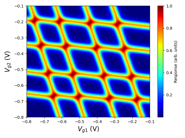
Fig. 4.11.1 Charge stability diagram showing Coulomb blockade diamonds, where each diamond corresponds to a charge configuration of the double-dot.
4.12. Full code
__copyright__ = "Copyright 2022-2026, Nanoacademic Technologies Inc."

from qtcad.device import materials as mt
from qtcad.device import io
from qtcad.device.mesh3d import Mesh, SubMesh
from qtcad.device import Device, SubDevice
from qtcad.device.many_body import Solver as ManyBodySolver
from qtcad.device.many_body import SolverParams as ManyBodySolverParams
from qtcad.device.schrodinger import Solver as SchrodingerSolver
from qtcad.device.schrodinger import SolverParams as SchrodingerSolverParams
from qtcad.transport.junction import Junction
from qtcad.transport.mastereq import add_spectrum
import numpy as np
from pathlib import Path
from matplotlib import pyplot as plt

script_dir = Path(__file__).parent.resolve()
mesh_dir = script_dir / "meshes"
mesh_file_dir = mesh_dir / "refined_gedqd.msh"
xao_dir = mesh_dir / "ge_dqd.xao"
out_dir = script_dir / "output"
out_dir.mkdir(exist_ok=True)

scaling = 1e-9  # nanometers
mesh = Mesh(scaling, mesh_file_dir)

dvc = Device(mesh, conf_carriers="h", hole_kp_model="luttinger_kohn_foreman")
dvc.set_temperature(0.1)

# Assign the material to regions
dvc.new_region("substrate", mt.SiGe_DFT)
dvc.new_region("SiGe_barrier", mt.SiGe_DFT)
dvc.new_region("Ge_well", mt.Ge)
dvc.new_region("SiGe_cap", mt.SiGe_DFT)
dvc.new_region("oxide", mt.Al2O3)

# Dot-region volumes
dvc.new_region("Ge_well.dot_region", mt.Ge)
dvc.new_region("SiGe_barrier.dot_region", mt.SiGe_DFT)
dvc.new_region("SiGe_cap.dot_region", mt.SiGe_DFT)

# boundary conditions
Ew = mt.Ge.chi + 1.1 * mt.Ge.Eg
dvc.new_gate_bnd("P1", -0.6, Ew)
dvc.new_gate_bnd("P2", -0.6, Ew)
dvc.new_gate_bnd("BC", 0.9, Ew)
dvc.new_gate_bnd("BL", 0.5, Ew)
dvc.new_gate_bnd("BR", 0.5, Ew)

dot_region_list = [
    "Ge_well.dot_region",
    "SiGe_barrier.dot_region",
    "SiGe_cap.dot_region",
]

dvc.set_dot_region(dot_region_list)

phi = io.load(out_dir / "electrostatic_potential.hdf5")
dvc.set_potential(phi)

dvc.set_V_from_phi()

submesh = SubMesh(dvc.mesh, dot_region_list)
subdvc = SubDevice(dvc, submesh)

schrodinger_params = SchrodingerSolverParams()
schrodinger_params.num_states = 20
schrodinger_params.tol = 1e-5

schrodinger_solver = SchrodingerSolver(subdvc, solver_params=schrodinger_params)
schrodinger_solver.solve()

subdvc.print_energies()
energies = subdvc.energies

many_body_solver_params = ManyBodySolverParams()
many_body_solver_params.n_degen = 1
many_body_solver_params.num_states = 8

slv = ManyBodySolver(subdvc, solver_params=many_body_solver_params)

coulomb_overlap = slv.get_coulomb_matrix(overlap=True, verbose=True)
np.save(out_dir / "coulomb_mat_overlap.npy", coulomb_overlap)

temperature_spec = 10  # Kelvin

lever_arm_matrix = np.load(out_dir / "lever_arm_matrix.npy")

gate_labels = ["BL", "P1", "P2", "BR"]

many_body_solver_params.energies = energies
many_body_solver_params.overlap = True
many_body_solver_params.coulomb_mat = coulomb_overlap
many_body_solver_params.alpha = lever_arm_matrix

jc = Junction(
    many_body_solver_params=many_body_solver_params,
    temperature=temperature_spec,
    contact_labels=gate_labels,
)


def get_add_spectrum(junc, gate_labels, gate_biases, temperature, verbose=True):

    junc.set_biases(gate_labels, gate_biases, verbose=verbose)
    out = add_spectrum(junc, temperature=temperature)
    return out


# set the bounds for the sweep
gate_1_min = -0.2
gate_1_max = 0.5
gate_2_min = -0.2
gate_2_max = 0.5

gate_1_biases = np.linspace(gate_1_min, gate_1_max, 90)
gate_2_biases = np.linspace(gate_2_min, gate_2_max, 90)

add_spectrum_mat = np.zeros((len(gate_1_biases), len(gate_2_biases)))

for idx_1, gate_1_bias in enumerate(gate_1_biases):
    for idx_2, gate_2_bias in enumerate(gate_2_biases):
        add_spectrum_mat[idx_1, idx_2] = get_add_spectrum(
            jc,
            gate_labels,
            np.array([0, gate_1_bias, gate_2_bias, 0]),
            temperature_spec,
            verbose=False,
        )

        np.savetxt(out_dir / "addition_spectrum.txt", add_spectrum_mat)

add_spec_to_plot = np.flip(np.transpose(add_spectrum_mat), axis=0)

fig, axs = plt.subplots()
axs.set_xlabel("$V_{g1}$ (V)", fontsize=16)
axs.set_ylabel("$V_{g2}$ (V)", fontsize=16)

diff_conds_map = axs.imshow(
    add_spec_to_plot / np.max(add_spec_to_plot),
    cmap="jet",
    interpolation="bilinear",
    extent=[gate_1_min - 0.6, gate_1_max - 0.6, gate_2_min - 0.6, gate_2_max - 0.6],
    aspect="auto",
)

fig.colorbar(diff_conds_map, ax=axs, label="Response (arb. units)")
fig.tight_layout()
fig.savefig(out_dir / "charge_stability_diagram.png")
plt.show()