4. Design and Maxwell eigenmode extraction of an flip-chip using Quantum Metal
4.1. Requirements
4.1.1. Software components
QTCAD®
Quantum Metal
4.1.2. Python script
qtcad/examples/tutorials/quantum_metal_flip-chip_eigenmodes.py
4.1.3. References
4.2. Briefing
In this example, we will design with Quantum Metal a flip-chip device consisting of an Xmon on one chip (the Q-chip) and a meandered CPW resonator on the other (the C-chip) and compute the system’s Maxwell eigemodes using our QTCAD renderer. Such a configuration, allows separation of the noisy readout and control lines (C-chip) from the qubits (Q-chip).
As in the other tutorials, the Josephson junction of the Xmon is approximated as an inductive lumped port.
Note
When running Quantum Metal simulations, make sure the Conda environment where Quantum Metal was set up is active, not the one in which QTCAD was installed.
If Quantum Metal was installed following Additional installation instructions for Quantum Metal, the
name of the activated environment will be quantum-metal.
In this case, this environment can be activated using
conda activate quantum-metal
Note
The Qiskit Metal project was recently rebranded as Quantum Metal.
Below, we import quantum_metal, but importing qiskit_metal is also
possible.
4.3. Mesh generation
As with the other tutorials involving Quantum Metal, the mesh and raw geometry files are generated on-the-fly using Quantum Metal.
Note
We leverage Quantum Metal’s Gmsh renderer to create meshes, so any device design supported by it will work with the QTCAD renderer.
4.4. Geometry of the problem
In the flip-chip configuration of this tutorial, the C-chip comprises a single readout resonator and the Q-chip comprises a single Xmon, with the superconducting (SC) sheets being modelled as 2D surfaces. Also, the chips will be separated by 10 μm and their Si substrates will have the same thickness of 280 μm.
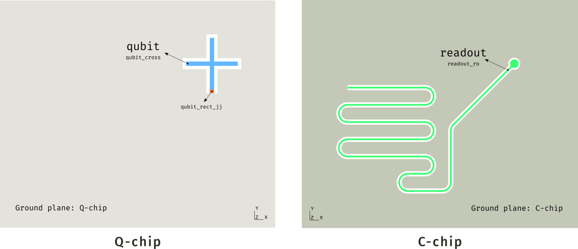
Fig. 4.4.11 Overview of the flip-chip device designed using Quantum Metal, each chip is shown individually. The different components labelled as follows: large type refers to the name of that component within Quantum Metal and smaller type refers to the physical group associated with that component in the mesh and geometry files.
4.5. Setting up the device
4.5.1. Preamble, file paths and base simulation parameters
We start by importing all relevant modules.
"""
Maxwell eigenmode extraction for a flip-chip device designed using Quantum Metal,
featuring an Xmon qubit on the Q-chip (layer 1) and a readout resonator on the C-chip
(layer 2) coupling capacitively face-to-face.
"""

from pathlib import Path

# Import Quantum Metal.
from quantum_metal import designs
from quantum_metal.qlibrary.resonators.readoutres_fc_generalized import (
    GeneralizedReadoutResFC,
)
from quantum_metal.qlibrary.qubits.transmon_cross import TransmonCross

# Import the QTCAD renderer.
from quantum_metal.renderers.renderer_qtcad.qtcad_renderer import QQTCADRenderer
We also define the working directory and relevant file paths.
# Directories and file paths.
device_name = "quantum_metal-flip-chip-eig"
# Work in the outputs folder of the current directory.
output_dir = str(Path(__file__).parent.resolve() / "output" / device_name)
# Geometry XAO file required for adaptive meshing.
geo_filepath = output_dir + "/" + device_name + ".xao"
# Mesh file.
mesh_filepath = output_dir + "/" + device_name + ".msh4"
We further define variables to control the adaptive meshing tolerance on the frequency and the characteristic lengths of the mesh.
# Adaptive meshing relative tolerance.
tolerance_relative = 0.05
# Set minimum and maximum characteristic lengths for the mesh elements.
mesh_h_min = "150um"
mesh_h_max = "500um"
Let us also define how many eigenmodes are to be extracted and the inductance of the Josephson junction.
# Number of Maxwell eigenmodes.
num_modes = 2
# Tunnelling junction inductance (in henries).
inductance = 14e-9
4.5.2. Creating the design object
To start the design process, we need to first instantiate a flip-chip design
object.
It comprises two chips: the Q-chip (labelled Q_chip, which we will
associated with layer 1) and the C-chip (labelled C_chip, which we will
associated with layer 2).
# Instantiate a flip-chip design object: Q_chip, C_chip.
design = designs.DesignFlipChip()
4.5.3. General geometry parameters
We can then define some general parameters related to the flip-chip geometry and the surrounding air box, and modify the design object accordingly.
Namely, let us define the desired gap between the chips, the thickness of the substrates and the air box parameters. Also, we leverage the fact that Quantum Metal allows simple arithmetic when parsing values
# Size/length variables for the chips/dielectric substrates.
# · Separation between the Q-chip and the C-chip.
chip_separation = "10um"
chip_separation_float = design.parse_value(chip_separation)
design.chips["C_chip"]["size"]["center_z"] = design.parse_value(f"-{chip_separation}/2")
design.chips["Q_chip"]["size"]["center_z"] = design.parse_value(f"+{chip_separation}/2")

# · Extrusion parameters / dielectric-substrate thickness.
chip_thickness = "280um"
# When setting the thicknesses of the dielectric holders, we need to use relative coordinates.
# That is, for the C-chip it must be negative.
design.chips["C_chip"]["size"]["size_z"] = design.parse_value(f"-{chip_thickness}")
design.chips["Q_chip"]["size"]["size_z"] = design.parse_value(f"+{chip_thickness}")

# Size/length variables for the air box (bottom and top padding).
# · Vertical distance of the airbox from the edge of the dielectric substrate.
airbox_z_buffer = "0.25mm"
# · Derive the desired distance from the z=0 plane.
#   (Quantum Metal allow simple arithmetic operations.)
airbox_padding = f"{chip_thickness} + {airbox_z_buffer} + {chip_separation}/2"
design.variables["sample_holder_top"] = design.parse_value(airbox_padding)
design.variables["sample_holder_bottom"] = design.parse_value(airbox_padding)
4.5.4. Adding the components
Before adding the different components, we define their labels. We also specify the coordinates of our Xmon.
# Define labels for the different components.
transmon_label = "qubit"
readout_label = "readout"

# Origin of the Xmon.
transmon_pos_x = "0um"
transmon_pos_y = "0um"
Then, we define a dictionary to store the different options for the Xmon.
Here, we place it on the Q-chip (Q_chip, layer 1).
# Define a dictionary with the parameters associated with the Xmon qubit.
options_transmon = dict(
    chip="Q_chip",
    layer="1",
    # Position of the geometric centre of the island relative to the origin.
    pos_x=transmon_pos_x,
    pos_y=transmon_pos_y,
    # Length of the ‘arms’ of the island.
    cross_length="150um",
    # Width of the ‘arms’ of the island.
    cross_width="25um",
    # Gap between the island and the ground plane.
    cross_gap="20um",
    # Anticlockwise orientation.
    orientation="90",
)
We do the same for the resonator, which is placed on the C-chip (C_chip,
layer 2) and couples capacitively to the Xmon across the flip-chip gap.
# Define a dictionary with the parameters associated with the readout resonator.
options_readout = dict(
    chip="C_chip",
    layer="2",
    # Position it on top of the center of the Xmon.
    pos_x=transmon_pos_x,
    pos_y=transmon_pos_y,
    # Radius of the circular open-to-ground termination of the resonator.
    readout_radius="25 um",
    # Width of the CPW center pin.
    readout_cpw_width="10 um",
    # Size of the gap to the surrounding ground plane.
    readout_cpw_gap="10 um",
    readout_cpw_turnradius="50 um",
    # Lengths of various parts of the CPW.
    readout_l1="500 um",
    readout_l2="300 um",
    readout_l3="200 um",
    readout_l4="100 um",
    readout_l5="450 um",
    # Length of a line that approximates an arc.
    arc_step="5 um",
    # By default, the `(Generalized)ReadoutResFC` components are right-aligned.
    mirror_x=True,
    start_angle=-45,
)

# Define the list of open-to-ground components.
open_pins = []
Note that we use the GeneralizedReadoutResFC custom component in this
tutorial.
An overview of it is found in the screenshot below.
More information can be found by inspecting its docstring.
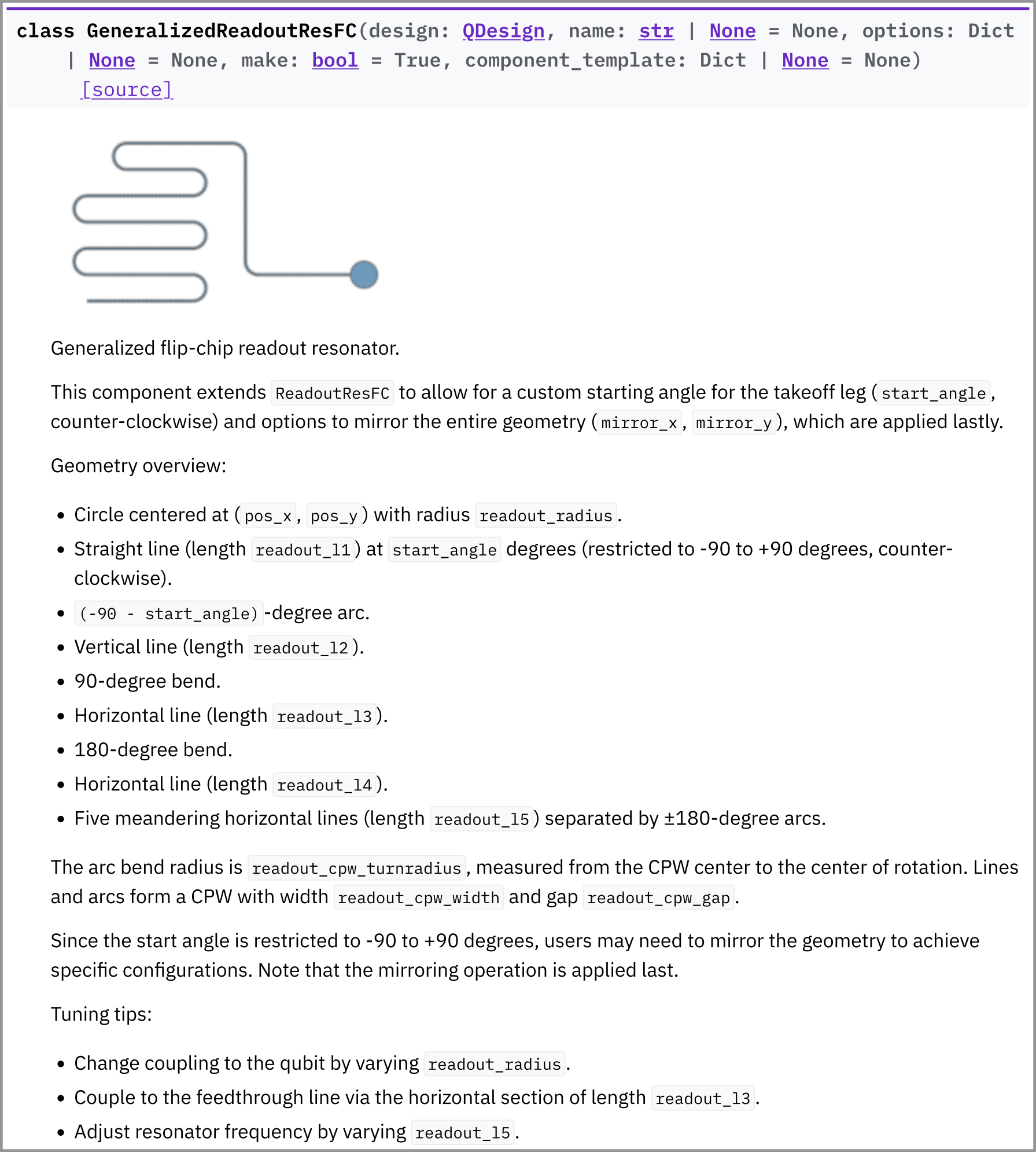
Fig. 4.5.7 Docstring of the GeneralizedReadoutResFC component.
We then include the components in the design.
# Add the different components to the design.
qubit = TransmonCross(design, transmon_label, options=options_transmon)
readout = GeneralizedReadoutResFC(design, readout_label, options=options_readout)
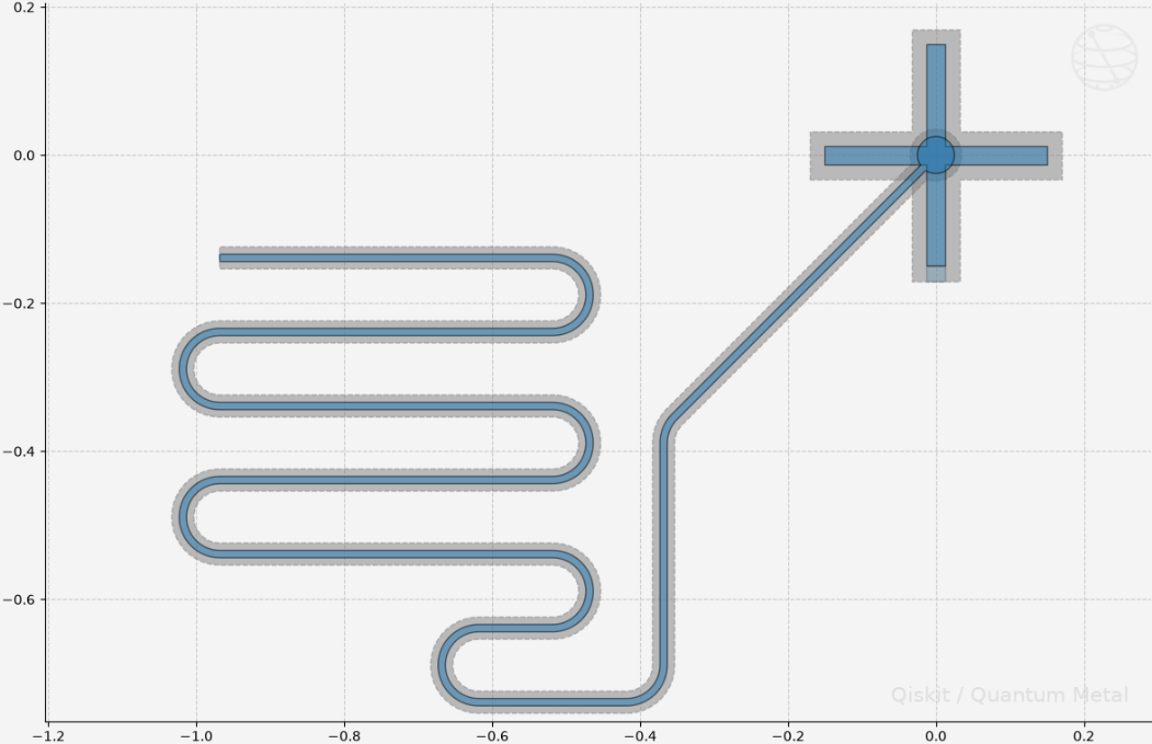
Fig. 4.5.8 Layout of the flip-chip device as shown in Quantum Metal.
4.5.5. Configuring the QTCAD renderer
Having created our device, we instantiate and configure our QTCAD renderer and the eigenmode solver.
Here, we use maxwell_emode_raw, which allow us to pass arguments directly
to QTCAD’s eigenmode solver.
Specifically, we set min_freq to \(1 \text{ GHz}\), which reduces the
time taken in the first AMR pass, as the lower bound for the eigenmode
frequencies does not need to be estimated automatically.
# Setting up the solver
qtcad_renderer = QQTCADRenderer(
    design,
    options=dict(
        adaptive=True,
        output_dir=output_dir,
        mesh_scale=1e-3,
        adaptive_mesh_scale=1e-3,
        geo_filepath=geo_filepath,
        mesh_filepath=mesh_filepath,
        make_subdir=False,
        maxwell_emode_raw=dict(
            num_modes=num_modes,
            tol_rel=tolerance_relative,
            min_freq=1e9,
        ),
    ),
)
4.5.6. Set up of the Josephson junction, rendering and meshing the design
Let us then render the device.
# Create the geometry from the design.
qtcad_renderer.render_design(
    open_pins=open_pins,
    # Render the Josephson junction.
    skip_junctions=False,
    # Do not mesh the device (yet).
    mesh_geoms=False,
    initial_mesh_h_min=mesh_h_min,
    initial_mesh_h_max=mesh_h_max,
)
Next, we set up the Josephson junction as an inductive port with linear
inductance via QQTCADRenderer.set_up_junction.
# Length of the junction: gap between the island and the ground plane.
length = options_transmon["cross_gap"]

# Add the tunneling junction.
table_junctions = qtcad_renderer.set_up_junction(transmon_label, inductance, length)
print(table_junctions)
        bnd_spec    inductance  length  width dir
0  qubit_rect_jj  1.400000e-08    0.02  0.025   x
Then, mesh the design and export the resulting geometry and mesh files.
# Mesh the device.
qtcad_renderer.gmsh.add_mesh(dim=3, intelli_mesh=False)

# Export the geometry and mesh files.
file_mesh, file_geo = qtcad_renderer.export_mesh()
4.5.7. Running the simulation
Finally, we can export the simulation parameters and compute the eigenmodes using QTCAD.
We also export a standalone script than can be used to (re)run the
eigenmode simulation directly using QTCAD via its own Conda environment.
This is especially useful if the user wants to modify the simulation set up or
post-processing directly, or use all QTCAD features – irrespective of their
support via QQTCADRenderer.
# Export parameters.
qtcad_renderer.export_parameters()
# Export standalone script.
qtcad_renderer.export_script("eigs")
# Run QTCAD to extract the Maxwell eigenmodes.
qtcad_renderer.run_qtcad("eigs")
Note
By default, it is assumed that you have installed QTCAD into a Conda environment named
qtcad. If not, when calling the methodrun_qtcad, make sure to pass the name of the appropriate Conda environment via the parameterenv_name. For instance, if QTCAD is installed in a Conda environment namedqtcad_sc, the call would beqtcad_renderer.run_qtcad("eigs", env_name="qtcad_sc").
To load the results, we use the method load_qtcad_maxwell_eigenmodes.
We also print the resulting frequencies, with 0 indexing the
fundamental-mode frequency of the system:
frequencies = qtcad_renderer.load_qtcad_maxwell_eigenmodes()
print(frequencies)
           Frequency (GHz)
Eigenmode
0                 4.132737
1                 7.123730
From the physics of the problem, the lower mode is expected to be associated with the Xmon and the higher one to describe an excitation of the resonator.
To verify that, we can inspect the electric field distribution using the method
plot_eigenmodes.
It generates a slice at a given z-coordinate (default: 0) of the absolute
value of the electric field from the VTU file output by QTCAD, which can
also be inspected using other software, for instance, ParaView.
qtcad_renderer.plot_eigenmodes(z=0, save=True)
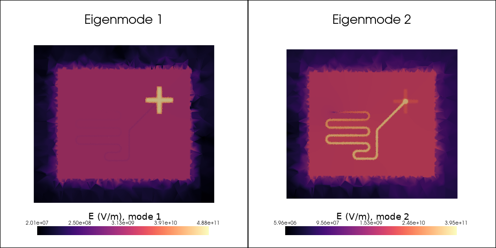
Fig. 4.5.9 Magnitude of the electric field – at the level of the ground plane, \(z=0\) – of the first two eigenmodes of the resonator-coupled Xmon system. The values are displayed in logarithmic scale.
Note
By default, the intensity plot is going to be shown, but not saved.
By passing save=True to plot_eigenmodes, the plot will be saved
and its path will be returned by the method, in addition to being
printed on screen.
By inspecting the distribution of the electric field, we find that the first mode is indeed associated with the Xmon qubit and the second mode is related to the fundamental resonance of the meandered resonator.
Furthermore, we can plot slices of specific modes using plot_eigenmode.
Let us then plot these modes individually, with the \(z\)-coordinate just
below the substrate of the chip associated with the resonant component.
qtcad_renderer.plot_eigenmode(n=1, z=1.01 * -chip_separation_float / 2, save=True)
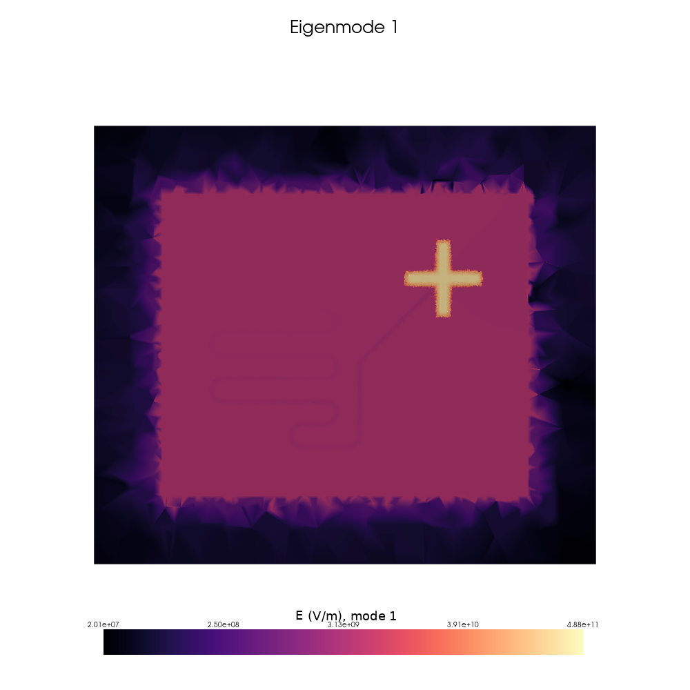
Fig. 4.5.10 Magnitude of the electric field – just below the Q-chip’s ground plane, inside the substrate – of the first eigenmode, associated with the Xmon, of the flip-chip system. The values are displayed in logarithmic scale.
qtcad_renderer.plot_eigenmode(n=2, z=1.01 * +chip_separation_float / 2, save=True)
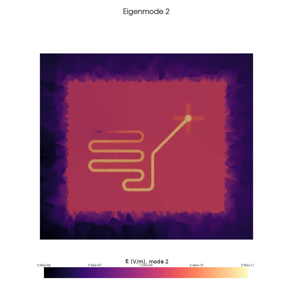
Fig. 4.5.11 Magnitude of the electric field – just below the C-chip’s ground plane, inside the substrate – of the second eigenmode, associated with the resonator, of the flip-chip system. The values are displayed in logarithmic scale.
4.6. Full code
__copyright__ = "Copyright 2022-2026, Nanoacademic Technologies Inc."

"""
Maxwell eigenmode extraction for a flip-chip device designed using Quantum Metal,
featuring an Xmon qubit on the Q-chip (layer 1) and a readout resonator on the C-chip
(layer 2) coupling capacitively face-to-face.
"""
from pathlib import Path

# Import Quantum Metal.
from quantum_metal import designs
from quantum_metal.qlibrary.resonators.readoutres_fc_generalized import (
    GeneralizedReadoutResFC,
)
from quantum_metal.qlibrary.qubits.transmon_cross import TransmonCross

# Import the QTCAD renderer.
from quantum_metal.renderers.renderer_qtcad.qtcad_renderer import QQTCADRenderer

# Directories and file paths.
device_name = "quantum_metal-flip-chip-eig"
# Work in the outputs folder of the current directory.
output_dir = str(Path(__file__).parent.resolve() / "output" / device_name)
# Geometry XAO file required for adaptive meshing.
geo_filepath = output_dir + "/" + device_name + ".xao"
# Mesh file.
mesh_filepath = output_dir + "/" + device_name + ".msh4"

# Adaptive meshing relative tolerance.
tolerance_relative = 0.05
# Set minimum and maximum characteristic lengths for the mesh elements.
mesh_h_min = "150um"
mesh_h_max = "500um"

# Number of Maxwell eigenmodes.
num_modes = 2
# Tunnelling junction inductance (in henries).
inductance = 14e-9

# Instantiate a flip-chip design object: Q_chip, C_chip.
design = designs.DesignFlipChip()

# Size/length variables for the chips/dielectric substrates.
# · Separation between the Q-chip and the C-chip.
chip_separation = "10um"
chip_separation_float = design.parse_value(chip_separation)
design.chips["C_chip"]["size"]["center_z"] = design.parse_value(f"-{chip_separation}/2")
design.chips["Q_chip"]["size"]["center_z"] = design.parse_value(f"+{chip_separation}/2")

# · Extrusion parameters / dielectric-substrate thickness.
chip_thickness = "280um"
# When setting the thicknesses of the dielectric holders, we need to use relative coordinates.
# That is, for the C-chip it must be negative.
design.chips["C_chip"]["size"]["size_z"] = design.parse_value(f"-{chip_thickness}")
design.chips["Q_chip"]["size"]["size_z"] = design.parse_value(f"+{chip_thickness}")

# Size/length variables for the air box (bottom and top padding).
# · Vertical distance of the airbox from the edge of the dielectric substrate.
airbox_z_buffer = "0.25mm"
# · Derive the desired distance from the z=0 plane.
#   (Quantum Metal allow simple arithmetic operations.)
airbox_padding = f"{chip_thickness} + {airbox_z_buffer} + {chip_separation}/2"
design.variables["sample_holder_top"] = design.parse_value(airbox_padding)
design.variables["sample_holder_bottom"] = design.parse_value(airbox_padding)

# Define labels for the different components.
transmon_label = "qubit"
readout_label = "readout"

# Origin of the Xmon.
transmon_pos_x = "0um"
transmon_pos_y = "0um"

# Define a dictionary with the parameters associated with the Xmon qubit.
options_transmon = dict(
    chip="Q_chip",
    layer="1",
    # Position of the geometric centre of the island relative to the origin.
    pos_x=transmon_pos_x,
    pos_y=transmon_pos_y,
    # Length of the ‘arms’ of the island.
    cross_length="150um",
    # Width of the ‘arms’ of the island.
    cross_width="25um",
    # Gap between the island and the ground plane.
    cross_gap="20um",
    # Anticlockwise orientation.
    orientation="90",
)

# Define a dictionary with the parameters associated with the readout resonator.
options_readout = dict(
    chip="C_chip",
    layer="2",
    # Position it on top of the center of the Xmon.
    pos_x=transmon_pos_x,
    pos_y=transmon_pos_y,
    # Radius of the circular open-to-ground termination of the resonator.
    readout_radius="25 um",
    # Width of the CPW center pin.
    readout_cpw_width="10 um",
    # Size of the gap to the surrounding ground plane.
    readout_cpw_gap="10 um",
    readout_cpw_turnradius="50 um",
    # Lengths of various parts of the CPW.
    readout_l1="500 um",
    readout_l2="300 um",
    readout_l3="200 um",
    readout_l4="100 um",
    readout_l5="450 um",
    # Length of a line that approximates an arc.
    arc_step="5 um",
    # By default, the `(Generalized)ReadoutResFC` components are right-aligned.
    mirror_x=True,
    start_angle=-45,
)

# Define the list of open-to-ground components.
open_pins = []

# Add the different components to the design.
qubit = TransmonCross(design, transmon_label, options=options_transmon)
readout = GeneralizedReadoutResFC(design, readout_label, options=options_readout)

# Setting up the solver
qtcad_renderer = QQTCADRenderer(
    design,
    options=dict(
        adaptive=True,
        output_dir=output_dir,
        mesh_scale=1e-3,
        adaptive_mesh_scale=1e-3,
        geo_filepath=geo_filepath,
        mesh_filepath=mesh_filepath,
        make_subdir=False,
        maxwell_emode_raw=dict(
            num_modes=num_modes,
            tol_rel=tolerance_relative,
            min_freq=1e9,
        ),
    ),
)

# Create the geometry from the design.
qtcad_renderer.render_design(
    open_pins=open_pins,
    # Render the Josephson junction.
    skip_junctions=False,
    # Do not mesh the device (yet).
    mesh_geoms=False,
    initial_mesh_h_min=mesh_h_min,
    initial_mesh_h_max=mesh_h_max,
)

# Length of the junction: gap between the island and the ground plane.
length = options_transmon["cross_gap"]

# Add the tunneling junction.
table_junctions = qtcad_renderer.set_up_junction(transmon_label, inductance, length)
print(table_junctions)

# Mesh the device.
qtcad_renderer.gmsh.add_mesh(dim=3, intelli_mesh=False)

# Export the geometry and mesh files.
file_mesh, file_geo = qtcad_renderer.export_mesh()

# Export parameters.
qtcad_renderer.export_parameters()
# Export standalone script.
qtcad_renderer.export_script("eigs")
# Run QTCAD to extract the Maxwell eigenmodes.
qtcad_renderer.run_qtcad("eigs")

frequencies = qtcad_renderer.load_qtcad_maxwell_eigenmodes()
print(frequencies)

qtcad_renderer.plot_eigenmodes(z=0, save=True)

qtcad_renderer.plot_eigenmode(n=1, z=1.01 * -chip_separation_float / 2, save=True)

qtcad_renderer.plot_eigenmode(n=2, z=1.01 * +chip_separation_float / 2, save=True)