3. Accuracy

In this section, we introduce common parameters influencing the accuracy of a calculation. The optimal value of certain parameters can be determined using physical reasoning whereas the optimal value of other parameters must be determined by trial and error.

3.1. Grid resolution

RESCU uses uniform Cartesian grids to discretize many quantities: the local pseudopotential, the pseudopotential projectors, the Hartree potential, the semi-local part of the exchange-correlation potential, the numerical atomic orbitals, the wavefunctions, etc. The accuracy of the numerical description of all these objects depends intrinsically on the underlying grid resolution. There are a few keywords to set the grid fineness in RESCU.

• domain.lowres A positive real number which corresponds to the distance between grid points along each dimension. This value is only a target since the actual resolution must yield an integer number of grid points along each direction. A typical value is 0.4 Bohr. This is the most transparent and preferred keyword to set the real space resolution.

• domain.cgridn A 1\(\times\)3 array of integers. It tells RESCU the number of grid points along each dimension. The user must be careful to choose a value which suits the lattice vectors and pseudopotentials. This keyword has precedence over domain.lowres.

Table 3.1.1 Allowed values for the keyword option.precision.

Prec.	Real grids	Planewave grids
Low	real-low	pw-low
Medium	real-med	pw-med
High	real-high	pw-high

In grid-based calculations (LCAO.status = false), several other keywords control precision: domain.highres (double-grid technique), interpolation.vloc (how to evaluate the local effective potential), interpolation.method, domain.vnlReal (non-local pseudopotential representation), etc. Non-experts need not worry about understanding and mastering all aspects of the algorithms used by RESCU, and hence it generally suffices to set domain.lowres along with option.precision which can take the values listed in Table 3.1.1. The values are quite self-explanatory. First, one may choose between real space and planewave grids. The former are more computationally efficient, but less precise at a fixed grid resolution. The latter may be competitive in smaller systems (say up to 100 atoms), but is simply too memory hungry in large systems (say more than 1000 atoms). Next, the precision of the grids (and the underlying computational methods) is controlled by means of low, med or high. Basically, the lower the precision, the lower the computational and memory requirements (again, this is true at a fixed grid resolution). To illustrate the above points, the total energy of the \(Au_4\) system as a function of resolution for various option.precision values is shown in Fig. 3.1.1.

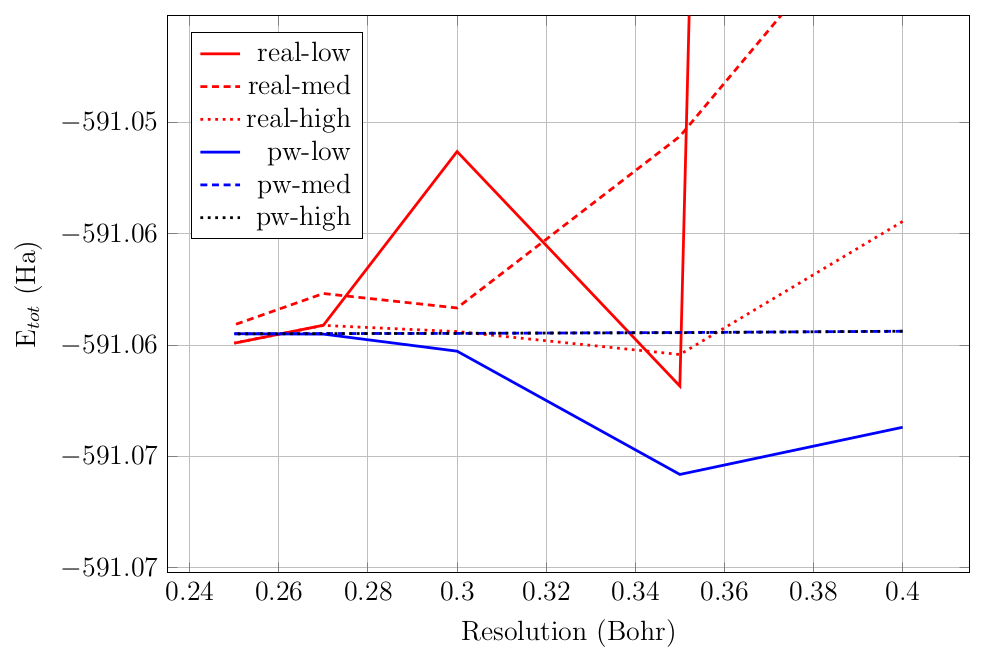
Fig. 3.1.1 Convergence of the total energy of the Au 4 system for various option.precision values.

3.2. Brillouin zone sampling

Periodic materials are usually simulated invoking Bloch’s theorem to divide the large (infinite) problem into independent subproblems (dependent on the crystal momentum) coupled via the density. For most purposes (e.g. band energy, density), averaging over the so-called first Brillouin zone is required, and hence the accuracy of the calculation depends directly on its sampling. RESCU implements an algorithm to generate Monkhorst-Pack grids. Such grids are \(\Gamma\)-centered for odd grid counts and shifted by half for even grid counts. The main control parameters are the following

• kpoint.gridn is a 1\(\times\)3 integer array defining the number of grid points along each dimension.

• kpoint.shift is also a 1\(\times\)3 array allowing the user to apply a global shift on the Monkhorst-Pack grid. Note that \(\Gamma\)-centered even numbered grids can be obtained setting kpoint.shift equal to [0.5 0.5 0.5].

• kpoint.sampling determines the scheme used to calculate the density of states, occupancy, etc. The allowed values are fermi-dirac, gauss, methfessel-paxton, tetrahedron and tetrahedron+blochl which are self-explanatory. While fermi-dirac and gauss are generally appropriate for \(\Gamma\)-point calculations, methfessel-paxton is suitable for metals and other systems with a nontrivial density of states at the Fermi energy. The tetrahedron method is applicable as long as there are more than four k-points and it is implemented following Blöchl’s method [BJA94]. If kpoint.sampling is equal to tetrahedron+blochl, second order corrections to the Fermi energy are included in the calculation of the occupancies.

• kpoint.sigma determines the width of the density of states’ shape functions (the shape of a single energy level). This is only pertinent if kpoint.sampling is equal to fermi-dirac, gauss or methfessel-paxton. Convergence may be unattainable if this value is too small (the default value is 0.001 Hartree). The units can be controlled using units.kpoint.sigma.

• kpoint.mpord sets the order of the Methfessel-Paxton shape functions.

3.3. Pseudopotentials

The fidelity of the pseudo-potential depends directly on the completeness of the projectors of the non-local component. By default, RESCU will use all projectors found in a pseudopotential file. Nevertheless, the principal quantum number and orbital angular momenta can be controlled using the keywords element.vnlNcutoff and element.vnlLcutoff respectively.

3.4. Atomic orbital basis

The Nanoacademic pseudopotential database files generally include a set of polarized double-zeta orbitals generated following the SIESTA method [SAGG02]. When doing numerical atomic orbital (NAO) calculations, it is crucial to have a basis which approximately spans the Kohn-Sham occupied subspace and the ground-state density. By default, RESCU will use all orbitals found in a pseudopotential file. However, it is possible to constrain the atomic basis of an element (e.g. to check convergence in the basis size) using the keywords element.aoLcutoff and element.aoZcutoff. Those limit the orbital angular momentum and \(\zeta\)-number of the basis functions respectively.

[BJA94]

Peter E. Blöchl, O. Jepsen, and O. K. Andersen. Improved tetrahedron method for Brillouin-zone integrations. Phys. Rev. B 49 (23 June 1994), pp. 16223–16233.

[SAGG02]

José M Soler, Emilio Artacho, Julian D Gale, Alberto Garcı́a, Javier Junquera, Pablo Ordejón, and Daniel Sánchez-Portal. The SIESTA method for ab initio order- N materials simulation. Journal of Physics: Condensed Matter 14.11 (2002), p. 2745.