7. Boundary conditions (Poisson’s equation)

RESCU is a real space DFT code, which allows it to implement various types of boundary conditions. RESCU currently supports three types of boundary conditions: Dirichlet, periodic and Neumann. The chosen boundary type is applied in solving the Poisson equation. The boundary type for other quantities, such as the wavefunctions, is inferred (see Table 7.1). In this section, we describe each type of boundary condition, discuss their purpose and demonstrate their usage.

The domain is always defined in terms of three lattice vectors (domain.latvec). A boundary condition type may be specified along each direction using the keyword domain.boundary. Note, however, that only periodic directions are allowed to be nonorthogonal. For instance, in a 2D hexagonal heterostructure, domain.boundary = [1,1,2] (periodic,periodic,Neumann) is valid provided that the third lattice vector is perpendicular to the first two. The default boundary condition for every direction is periodic (1). In the following sections, we provide specific details for each boundary condition type.

Table 7.1 Boundary condition types. The value of domain.boundary is indicated in the parenthesis. The second column indicates the boundary condition imposed on the Hartree potential (obtained by solving the Poisson equation). The third column indicates the boundary condition imposed on the wavefunctions. For the periodic boundary condition, the 0 and 1 subscript indicate the lower and upper boundaries along a given direction.
BC	Potential \(v_H\)	Wavefunctions \(\psi\)
Dirichlet	\(v_H(\partial\Omega) = f_{input}(\partial\Omega)\)	\(\psi(\partial\Omega) = 0\)
Periodic	\(v_H(\partial\Omega_0) = v_H(\partial\Omega_1)\)	\(\psi(\partial\Omega_0) = \psi(\partial\Omega_1)\)
Neumann	\(\partial v_H(\partial\Omega)/\partial x_i = 0\)	\(\psi(\partial\Omega) = 0\)
Open	\(v_H(\partial\Omega) = \int dr' \rho(r')/\|r-r'\|\)	\(\psi(\partial\Omega) = 0\)
Dirichlet	\(v_H(\partial\Omega) = \int dr' \rho(r')/\|r-r'\| \\[-2ex] + f_{input}(\partial\Omega)\)	\(\psi(\partial\Omega) = 0\)

7.1. Periodic (1)

Periodic boundary conditions are enforced by default on both the Hartree potential and the wavefunctions. This boundary condition type should be used in crystals. It may also be used to simulate open boundary conditions through the use of supercell geometries, albeit this is suboptimal in terms of efficiency. When using mixed boundary conditions, e.g. for a slab simulation, the keyword domain.boundary must be set to 1 along the periodic directions (as determined in domain.latvec). Consider the following (partial) input file

domain.latvec = [100 7.0 0.0
                 7.0 100 0.0
                 0.0 0.0 10]
domain.boundary = [1 1 2]

This tells RESCU that the domain is a flat and large monoclinic cell. The first two dimensions are nonorthogonal, which is allowed since both are periodic. The third dimension is nonperiodic (Neumann), which again is allowed since the third lattice vector is perpendicular to the first two.

7.2. Neumann (2)

The 2D periodic + 1D open geometry is frequently encountered (in suspended two-dimensional crystals for example). This geometry often result in the system having a significant global dipole moment, an artifact of the infinite in-plane dimensions. The Hartree potential then tends to different values on each side of the system in the perpendicular dimension. If periodic boundary conditions are enforced, the Hartree potential is linear in the vacuum region, with a slope that is inversely proportional to the vacuum size. The convergence of the Hartree potential is thus very slow when adopting the supercell method.

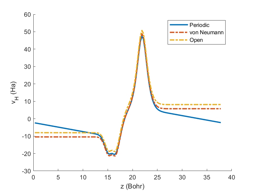
Fig. 7.2.1 Average Hartree potential of a graphene-boron-nitride heterostructure with respect to the z-coordinate. The Hartree potential is average in the in-plane directions. The blue curve represents the Hartree potential as calculated in a periodic supercell. The periodic boundary conditions force a linear potential in the vacuum region. The orange curve represents the Hartree potential as calculated with homogeneous Neumann boundary conditions. The potential then quickly settles to constant values on either side of the heterostructure. The yellow curve represents the Hartree potential as calculated with open boundary conditions.

The situation is remedied by adopting homogeneous Neumann boundary conditions along the perpendicular dimension when solving the Poisson equation. Simply put, this means that the Hartree potential derivative is set to zero on the domain boundary. Indeed, at a sufficient distance, we expect the Hartree potential (of a neutral system) to reach a constant. In this way, the Poisson equation is well defined and the constant on either side of the structure is allowed to differ, thereby removing the artificial linear potential between the images. In several planewave codes, this is referred as dipole correction. Apart from dealing with the global dipole moment, Neumann boundary conditions usually allow reducing the size of the vacuum used in a simulation, which may lead to significant computational gains. An example is found in Fig. 7.2.1 where is depicted the Hartree potential of a graphene-boron-nitride heterostructure as calculated by periodic and Neumann boundary conditions.

We stress that Neumann boundary condition are only enforced upon the Hartree potential. The wavefunctions should be confined to the structure along the nonperiodic dimension, they should decay to zero at the domain boundary. Mathematically, this means that homogeneous Dirichlet boundary conditions are imposed upon the wavefunctions (see Table 7.1). This in turns result in homogeneous Dirichlet boundary conditions for the density.

Another point of caution is that the absolute value of the electrostatic potential is (conventionally) set to zero. This is consistent with the case of fully periodic boundary conditions. Practically, this means that the relative vacuum values of the Hartree potential are independent of the vacuum thickness (beyond a certain vacuum thickness), but their absolute values vary such as to maintain an average electrostatic potential of zero.

Finally, as mentioned in the previous section, Neumann boundary conditions can be imposed along a direction by setting the keyword domain.boundary to 2.

7.3. Induced Dirichlet (0)

Certain simulations demand imposing a specific boundary value to the Hartree potential. The corresponding type of boundary condition is called Dirichlet. This can be useful in simulating a gate nonatomistically, for instance. Note that specifying a value on the boundary is tantamount to enforcing an induced field, not an external field. As in the case of Neumann boundary conditions, the wavefunctions should be confined to the structure along the nonperiodic dimensions, and hence they satisfy homogeneous Dirichlet boundary conditions.

Dirichlet boundary conditions are selected by setting the keyword domain.boundary to 0. By default, the boundary values are set to zero. In general, the boundary values along the first, second and third lattice vectors are specified using the keywords domain.bvalx, domain.bvaly and domain.bvalz respectively. Without loss of generality, let’s consider domain.bvalz. The values on the lower and upper boundaries are passed via a cell array, denote by curly braces. The value on a boundary can be specified in three ways:

If the value on a boundary is constant, it can be specified as a simple number;
If the value on a boundary is function with an analytical form, it can be specified as a function handle which evaluates the function. Note that function handle should evaluate a function of two variables on the domain \([0,1]\times[0,1]\) in general;
If the value on a boundary is numeric-valued function, the function can be read from a MAT-file. The path of the MAT-file containing the function values should be passed as a string. The function values should be arranged in an array that has the exact shape of the boundary in question. The exact name of the variable is unimportant, but the variable should be lone in the MAT-file. For instance, the lower y-boundary of a [20,30,40] points domain (domain.cgridn) should be an array of size [20,1,40].

We close this section with the following example

domain.latvec = [100 7.0 0.0
                 7.0 100 0.0
                 0.0 0.0 5]
domain.boundary = [1,1,0]
domain.bvalz = {'bvalz0.mat' @(u,v) exp(-((u-0.5).^2 + (v-0.5).^2)/0.05)}
domain.cgridn = [200,200,10]

Dirichlet boundary conditions are imposed along the z-direction of this monoclinic unit cell. The value on the lower boundary is specified by an array stored in bvalz0.mat. Here the array is \(200\times 200\), so it is convenient to define the grid by hand using the keyword domain.cgridn. Adjusting domain.lowres to yield a \(200\times 200\times 10\) grid may be difficult. The value on the upper boundary, of cylindrical Gaussian shape, is specified by a function handle. A word of caution, the boundary values of a given direction should respect the boundary conditions along the remaining directions as possible. Here, the Gaussian function violates the periodic boundary conditions along the xy-directions. However, its width is sufficiently small for it to approximately respect periodic boundary conditions.

7.4. Open (3)

If one of the dimensions is open while the other two are periodic, then the potential on the open boundary can be calculated exactly (7.4.1).

(7.4.1)\[v_H(\mathbf{r},z) = \sum\limits_{z_i\in \mathcal{H}_i} -2\pi\rho_\mathbf{0}(z_i)|z-z_i| + 2\pi \sum\limits_{\mathbf{k}}^{'}e^{i\mathbf{k}\cdot\mathbf{r}} \frac{\rho_\mathbf{k}(z_i)}{k} e^{-|k||z-z_i|}\]

If two of the dimensions are open while the other is periodic, then the potential on the open boundary can be calculated using (7.4.2).

(7.4.2)\[v_H(x,y,z) = \sum\limits_{x_i,y_i\in \mathcal{H}_i} -2\log(d_{i}(x,y)) \rho_\mathbf{0}(x_i,y_i) + 2 \sum\limits_{k}^{'}e^{ikz} K_0(d_{i}(x,y)k) \rho_k(x_i,y_i)\]

where \(d_{i}(x,y) = \sqrt{(x-x_i)^2+(y-y_i)^2}\) and \(K_0\) is the decaying modified Bessel function. After calculating the Hartree potential on the boundary, the equation can be solved using it as a regular Dirichlet boundary condition. This is done by setting the value of the keyword domain.boundary equal to 3 for the corresponding dimension. As can be seen in Fig. 7.2.1, the transverse-averaged Hartree potential calculated using open boundary conditions matches the one calculated with Neumann boundary conditions, albeit with a global shift. This is because the Neumann absolute level is chosen such that the average potential is zero while it is calculated from (7.4.1) in the former case. Note that unlike homogeneous Neumann boundary conditions, open boundary conditions can capture all multipole moments of a slab sytems and not only the perpendicular dipole moment.

7.5. External Dirichlet (4)

Often, the external field should be specified instead of the induced field. In this case, domain.boundary should be set to 4 instead of 0. This calculation requires calculating the potential on the open boundaries, and hence the same restrictions as open boundary calculations apply (one of the dimensions is open while the other two are periodic). The external field can be specified using domain.bvalx, domain.bvaly or domain.bvalz just like the type-0 Dirichlet boundary conditions.