20. Wannier function calculation
In this section we introduce maximally localized Wannier function (MLWF)
calculations [MV97, SMV01, AM12].
Following a self-consistent calculation, one obtains the ground-state
density, from which the Kohn-Sham (KS) states can be calculated. The KS
state basis is usually delocalized in real space and non-smooth in
reciprocal space, which is impractical for certain applications. It is
possible to derive a maximally localized basis from the canonical KS
states (or a subset of them), a procedure called gauge optimization
which yields the MLWF. Note that the MLWF solver is only implemented for
LCAO calculations (LCAO.status = true).
20.1. Example: MLWF of FCC copper
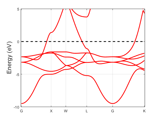
Fig. 20.1.1 Band structure of FCC copper.
Suppose we have completed a self-consistent calculation of face-centered
cubic copper and that the results are in ./results/cu_lcao_scf.h5
and ./results/cu_lcao_scf.mat. Following the instructions in section
Band structure calculation, we can produce a band structure which looks like
Fig. 20.1.1.
The self-consistent input file used to generate these results is shown below:
LCAO.status = 1
info.savepath = './results/cu_lcao_scf'
info.calculationType = 'self-consistent'
atom.element = 1
atom.fracxyz = [1 1 1]*0.5
domain.latvec = ~eye(3)/2*6.8314;
domain.lowres = 0.2
element(1).species = 'Cu'
element(1).path = './Cu_LDA_TM_DZP.mat'
functional.list = {'XC_LDA_X','XC_LDA_C_PW'}
mixing.tol = [1e-7 1e-7]
kpoint.gridn = [11 11 11]
force.status = false

% Wannier parameters
kpoint.shift = 0.5*mod(kpoint.gridn+1,2)
symmetry.pointsymmetry = false
symmetry.timereversal  = false
eigensolver.emptyBand  = 1000
We now compute the Wannier functions for the bands comprised in the
interval \([-6 -2]\). Create the input file cu_lcao_wan as
follows
info.savepath = './results/cu_lcao_wan'
info.calculationType = 'wannier'
rho.in = './results/cu_lcao_scf'
kpoint.gridn = [11 11 11]
units.energy = 'ev'
wannier.outwin = [-10  -1]
wannier.shiftEf = true
wannier.orbi = 6:10
then execute rescu
rescu -i cu_lcao_wan
The purpose of each keywords is mentioned hereafter
info.calculationTypeis set towannierso that RESCU computes MLWF;rho.inmust be the path to the self-consistent calculation results,./results/cu_lcao_scfin the present example;kpoint.gridndefines the reciprocal space grid. It is a \(1\times 3\) vector specifying the number of grid points in the direction of each reciprocal lattice vectors. It is recommended to use a grid as fine or finer than that used in the self-consistent calculation;units.energysets the default input energy unit to electronvolt;wannier.outwinspecifies the outer energy window. By default, the window is absolute and in units of Hartree. Here, the unit of energy is electronvolt as specified byunits.energyand the values are relative to the Fermi energy as specified bywannier.shiftEf. For every k-point, the MLWF calculator minimizes the spread functional within the subspace of the KS states comprises in the outer energy window. Too few or too many states can impede the optimization procedure. In the present case, we find that including the lowest \(s\)-band improves the MLWF description, and hence we set the lower window bound to (\(E_F-10\)) eV. The upper bound is not as important, but it should enclose all \(d\)-bands, so we set it to (\(E_F-1\)) eV;wannier.shiftEfis set totruesuch that the energies given bywannier.outwinare relative to the Fermi level;wannier.orbiis a vector of orbital indices that determines which orbitals to use as a projection basis. It is the most important keyword in Wannier function calculations. Firstly, the projection basis determines the dimensionality of the MLWF basis: one gets a MLWF for every projection orbital. It follows that the size of the Wannier Hamiltonian and other operators also has this dimensionality. Second, the projection basis provides an initial guess of sorts for the Wannier functions. It should thus be picked in accordance with the character of the bands in the target energy window, which can be determined from symmetry or physical intuition for example. Here, the bands in the given energy window have \(d\)-orbital character (as can be observed in a band decomposition calculation, section Band structure decomposition). Using the information inLCAO.orbInfo, we see that the orbitals indices corresponding to \(d\)-orbitals are 6:15, for a total of 10 orbitals since there is one \(\zeta_1\)-shell and one \(\zeta_2\)-shell each with 5 orbitals. We use the \(\zeta_1\)-orbitals, which have indices [6,7,8,9,10], as a projection basis since they have the largest weights in the band structure decomposition.
There are two keywords controlling KS subspace selection besides
wannier.outwin: wannier.innwin and wannier.bandi (which
stand for inner energy window and band index range respectively).
Copper being a metal, is has so-called entangled bands, which means that
it is not possible to isolate a subset of KS states and optimize the
spread functional with respect to a pure gauge transform. Semiconductors
however often have groups of bands isolated by energy gaps. It may then
be convenient to specify which bands to include in the KS subspace
specifying band indices instead of an energy window, hence the keyword
wannier.bandi. For example, to generate Wannier functions for the
four valence bands of silicon, we should set wannier.bandi = [1 4],
assuming no core states are included in the pseudopotential’s reference
configuration. A user may sometimes want to force the inclusion of
certain KS states in the outer energy window, which is achievable via
wannier.innwin.
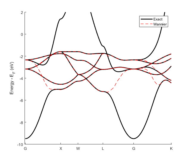
Fig. 20.1.2 Band structure of FCC copper in black. Wannier band structure of FCC copper in red.
The results of the Wannier function calculation are found in
results/cu_lcao_wan.mat and results/cu_lcao_wan_hamiltonian.wan.
The file results/cu_lcao_wan.mat contains the usual output data and
wannier.centersthe wannier function positions (centers);wannier.Ukthe unitary transforms to convert Bloch functions to Wannier functions and vice versa (\(U_{\mathbf{k}}\));wannier.Uk0the subspace projection transforms (\(U_{\mathbf{k}}^0\));wannier.hamthe displaced Hamiltonian in the Wannier function basis (\(H_{{\mathbf{R}}^W}\));wannier.vecthe Hamiltonian displacements (\(\mathbf{R}\)).
The \(\mathbf{k}\)-dependent Wannier functions can be recovered computing
where \(\psi_{j}^{\mathbf{k}\sigma}\) are the canonical Kohn-Sham states, and the MLWF computed by Fourier transform
The Wannier representation of the Hamiltonian is found in
wannier.ham, but it is also saved in the Wannier90 code format in
results/cu_lcao_wan_hamiltonian.wan.
The Wannier band structure can be calculated creating the input
cu_lcao_wbs
rho.in = 'results/cu_lcao_wan'
info.savepath = './results/cu_lcao_wbs'
info.outfile = 'fcu_lcao_wbs.out'
info.calculationType = 'wannier-bs'
and passing it to RESCU
rescu -i cu_lcao_wbs
The result can be plotted as follows
rescu -p result/cu_lcao_wbs
The Wannier band structure by itself may look a bit strange, so it is usually represented contextually with the standard band structure as in Fig. 20.1.2.
Nicola Marzari and David Vanderbilt. Maximally localized generalized Wannier functions for composite energy bands. Physical Review B - Condensed Matter and Materials Physics, 56.20 (1997), pp. 12847–12865.
Ivo Souza, Nicola Marzari, and David Vanderbilt. Maximally localized Wannier functions for entangled energy bands. Physical Review B - Condensed Matter and Materials Physics 65.3 (2001), pp. 1–13.
Arash A. Mostofi et al. Maximally localized Wannier functions: Theory and applications. Reviews of Modern Physics 84.4 (Oct. 2012), pp. 1419–1475.