2. Output files guidelines
2.1. General output
Let’s say you completed a calculation specified by the following input file
info.calculationType = 'self-consistent'
info.savepath = './results/bn_real_scf'
info.outfile = 'fbn_real_scf.out'
element(1).species = 'B';
element(1).path = './B_AtomicData.mat'
element(2).species = 'N';
element(2).path = './N_AtomicData.mat'
alat = 6.85; % in bohr
atom.xyz = alat*[0 0 0;.25 .25 .25]
atom.element = [1;2]
domain.latvec = alat*[.5 .5 0;.5 0 .5;0 .5 .5]
domain.lowres = 0.2
functional.list = {'XC_GGA_X_PBE','XC_GGA_C_PBE'}
kpoint.gridn = [3 3 3]
kpoint.sigma = 0
mixing.tol = 1e-8*[1 1]
dos.status = 0
option.saveWavefunction = 1
The location of the output is determined by the keyword info.savepath = ./results/bn_real_scf.
RESCU output can be divided into two classes:
- Distributed
This includes essentially data structures living on some grid (describing real space or reciprocal space fields like the electron density, the Hartree potential, wavefunctions, etc.) and atomic orbital matrices (like the Hamiltonian). This is because in large scale systems, any of these quantities is potentially too large to fit in the memory of a single node.
- Global
This includes pretty much anything else, like the atomic coordinates, the lattice vectors, the total energy, etc.
The global quantities are included in the MAT file (in our example ./results/bn_real_scf.mat).
A MAT-file may be read simply with the MATLAB command load.
This is shown below.
>> load('/home/vincentm/Downloads/rescu-2.7.0/examples/results/al_lcao_scf.mat')
>> atom

atom =

struct with fields:

      Ztot: 3
      desc: [1×1 struct]
   element: 1
   nvalence: 3
         xyz: [0 0 0]

>> atom.desc

ans =

struct with fields:

   element: 'Vector containing the element index of every atoms.'
   nvalence: 'atom.nvalence determines the number of valence electrons in self-consistent calculations. The valence is intrinsically linked to the density. By default, atom.nvalence is determined such that the system is charge neutral. It is however possible to choose a value whereby the system is non-neutral.'
         xyz: 'Cartesian coordinates of every atoms in atomic units (Bohr radii).'
In each structure like atom, there is a desc field which contains descriptions
for the parameters and output data.
The distributed quantities are included in the HDF5 file (in our example ./results/bn_real_scf.h5).
HDF5 files may be parsed with h5disp and
read with h5read in MATLAB.
For example,
>> h5disp('results/al_lcao_scf.h5','/rho/rhoOut');
HDF5 al_lcao_scf.h5
Dataset 'rhoOut'
   Size:  729x1
   MaxSize:  729x1
   Datatype:   H5T_IEEE_F64LE (double)
   ChunkSize:  []
   Filters:  none
   FillValue:  0.000000
   Attributes:
      'real':  1.000000
2.2. Units
All output quantities are in atomic units, unless otherwise specified. This means that energies are in Hartree and lengths (area, volumes, etc.) are in Bohr. For example, one could revise the above input file as follows
units.length = 'ang'
alat = 3.6249 % in ang
atom.xyz = alat*[0 0 0;.25 .25 .25]
atom.element = [1;2]
domain.latvec = alat*[.5 .5 0;.5 0 .5;0 .5 .5]
The lattice constant is now passed in Angstroms, but the system specified by the input file is equivalent. In both cases, the output is in atomic units. For example, one could load and show the lattice vectors
>> load('/home/vincentm/repos/rescumat/tmp/results/bn_real_scf.mat')
>> domain.latvec

ans =

   3.4250    3.4250         0
   3.4250         0    3.4250
         0    3.4250    3.4250
2.3. Output control
As mentioned in section General output, output data can be quite demanding in terms of disk space, and hence not everything is stored on disk by default. The keywords in table Table 2.3.1 shows various keywords used to control which output data should be saved
Keywords |
Description |
HDF5 group |
|---|---|---|
option.saveDensity |
Density (electronic, atomic, etc.) |
|
option.saveDFPT |
DFPT parameters |
|
option.saveEigensolver |
Eigensolver parameters |
|
option.saveInterpolation |
Interpolation matrices |
|
option.saveLevel |
Set to 2 to save everything |
|
option.saveLCAO |
All LCAO parameters |
|
option.saveLcaoHam |
LCAO Hamiltonian |
|
option.saveMisc |
Debug option |
|
option.saveMixing |
Mixer history |
|
option.savePartialWeights |
Band decomposition |
|
option.savePotential |
Potential |
|
option.saveTau |
Kinetic energy density |
|
option.saveWavefunction |
Wavefunctions (periodic part) |
|
option.saveDensityMatrix |
Real space density matrix |
|
option.saveDensityMatrixK |
Density matrix (k-space) |
|
Local DOS |
|
|
dfpt.saveEPImat |
Electron-phonon matrix |
|
dfpt.saveElectronVelocity |
Electron velocities |
|
dfpt.saveElectronSE |
Electron self-energy (eph scattering) |
|
dfpt.saveElectronTau |
Electron lifetime (eph scattering) |
|
Mulliken population matrix |
|
Some quantities like the wavefunctions /waveFunction/psi have k-point and spin indices.
The HDF5 datasets are thus numbered consecutively from 1 to N to distinguish them.
The first \(n_k\) wavefunctions correspond to the first \(n_k\) irreducible
k-points specified in kpoint.ikdirect.
In collinear spin calculations, the \(n_k\) psi are for spin up and the next
\(n_k\) psi datasets are for spin down.
The same logic holds for other quantities like /LCAO/partialWeight.
2.4. Grids
In RESCU, there are generally two grids:
One for the wavefunctions, the so-called coarse grid with grid number given by
domain.cgridn;One for everything else, the so-called fine grid with grid number given by
domain.fgridn.
In many calculations (e.g. all LCAO calculations), these grids are the same. But in some cases, they might be different. So when reshaping a quantity like the density, you should pay attention to use the grid that matches the number of elements in the array.
Another important point is where the grid is with respect to the unit cell. In RESCU, the fractional coordinates of grid points along each dimension are \([du,1]\). Let’s say you want to work with the fine grid, you can thus get the 1D grids as follows
nu = domain.fgridn(1);  % # grid points along dimension #1
nv = domain.fgridn(2);  % # grid points along dimension #2
nw = domain.fgridn(3);  % # grid points along dimension #3
u2 = (1:nu)/nu;         % fractional coords of grid along lattice vector #1
v2 = (1:nv)/nv;         % fractional coords of grid along lattice vector #2
w2 = (1:nw)/nw;         % fractional coords of grid along lattice vector #3
The full 3D grid can be generated as follows
avec = domain.latvec;
[u2,v2,w2] = ndgrid(u2,v2,w2);
xyz = [u2(:) v2(:) w2(:)]*avec;
x = reshape(xyz(:,1), nu, nv, nw);
y = reshape(xyz(:,2), nu, nv, nw);
z = reshape(xyz(:,3), nu, nv, nw);
You can visualize this as follows
figure(); hold on
avec = domain.latvec;
plot_domain_edges(avec);
scatter3(x(:),y(:),z(:), 'filled')
and you’ll see something like figure Fig. 2.4.1
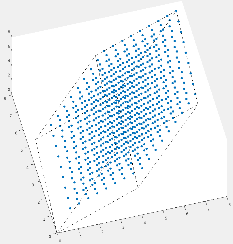
Fig. 2.4.1 Grids for an Al calculation. Note the grid starts at \(dx\) not 0.
2.5. Arrays
Many quantities are conveniently represented as arrays. For example, lattice vectors are written as
avec = [[1.,2.,3.];[4.,5.,6.];[7.,8.,9.]]
If arrays with more than one dimension are written as vectors, they will be reshaped automatically. RESCU (like MATLAB) uses the so-called Fortran order, which means that a vector is reshaped filling the 1st dimension, then the 2nd, then the 3rd etc. This means that
avec = [1.,2.,3.,4.,5.,6.,7.,8.,9.]
is reshaped to
avec = [[1.,4.,7.];[2.,5.,8.];[3.,6.,9.]]
which corresponds to a matrix
By contrast, there exist the so-called C ordering where multidimensional arrays are filled backward, i.e. starting by the last dimension.
This means that
avec = [1.,2.,3.,4.,5.,6.,7.,8.,9.]
is reshaped to
avec = [[1.,2.,3.];[4.,5.,6.];[7.,8.,9.]]
which corresponds to a matrix
Going back to the example above, suppose you import the density as
>> rho = h5disp('results/al_lcao_scf.h5','/rho/rhoOut');
    Dataset 'rhoOut'
     Size:  15625x1
     MaxSize:  15625x1
     Datatype:   H5T_IEEE_F64LE (double)
     ChunkSize:  []
     Filters:  none
     FillValue:  0.000000
     Attributes:
         'real':  1.000000
you should reshape rho according to the domain data in
results/al_lcao_scf.mat. In the present example, domain.fgridn = [9,9,9]
so rho = reshape(rho, [9,9,9]) will give you the density as a 3D array.
For the wavefunctions, you would see something like
>> h5disp('results/bn_real_scf.h5','/waveFunction' )
HDF5 bn_real_scf.h5
Group '/waveFunction'
   Dataset 'psi1'
      Size:  15625x12
      MaxSize:  15625x12
      Datatype:   H5T_IEEE_F64LE (double)
      ChunkSize:  []
      Filters:  none
      FillValue:  0.000000
      Attributes:
            'real':  1.000000
   Dataset 'psi2'
      Size:  15625x24
      MaxSize:  15625x24
      Datatype:   H5T_IEEE_F64LE (double)
      ChunkSize:  []
      Filters:  none
      FillValue:  0.000000
      Attributes:
            'real':  0.000000
Note that the datasets are not 1D but 2D now, with shape 15625x24.
The first index runs over the grid points and the second index is for
bands. There are therefore 24 bands of boron nitride in this output.
2.6. Normalization
In RESCU, fields are treated in analogy with analytical fields. This means that the normalization condition for the density, for instance, is
where \(\Omega\) is a unit cell and \(N_{el}\) is the number of electrons. Numerically, this translates to (for an aluminum primitive cell)
>> load('./results/al_lcao_scf.mat')
>> vol = abs(det(domain.latvec));
>> fn = prod(domain.fgridn);
>> dr = vol/fn;
>> rho = h5read('results/al_lcao_scf.h5','/rho/rhoOut');
>> sum(rho)*dr

ans =

   3.0000
Similarly, the normalization condition for wavefunctions, or wavefunction-like quantities like atomic orbitals, is
Numerically, this translates to (again for an aluminum primitive cell)
>> vol = abs(det(domain.latvec));
cn = prod(domain.cgridn);
dr = vol/cn;
psi = h5read('results/al_real_scf.h5','/waveFunction/psi1');
psi'*psi*dr

ans =

Columns 1 through 7

   1.0000   -0.0000   -0.0000   -0.0000    0.0000    0.0000   -0.0000
   -0.0000    1.0000   -0.0000   -0.0000    0.0000    0.0000    0.0000
   -0.0000   -0.0000    1.0000   -0.0000    0.0000    0.0000    0.0000
   -0.0000   -0.0000   -0.0000    1.0000   -0.0000   -0.0000    0.0000
   0.0000    0.0000    0.0000   -0.0000    1.0000    0.0000    0.0000
   0.0000    0.0000    0.0000   -0.0000    0.0000    1.0000   -0.0000
   -0.0000    0.0000    0.0000    0.0000    0.0000   -0.0000    1.0000
   -0.0000   -0.0000   -0.0000   -0.0000    0.0000   -0.0000   -0.0000
   -0.0000    0.0000   -0.0000   -0.0000   -0.0000   -0.0000   -0.0000
   -0.0000    0.0000    0.0000   -0.0000    0.0000   -0.0000    0.0000

Columns 8 through 10

   -0.0000   -0.0000   -0.0000
   -0.0000    0.0000    0.0000
   -0.0000   -0.0000    0.0000
   -0.0000   -0.0000   -0.0000
   0.0000   -0.0000    0.0000
   -0.0000   -0.0000   -0.0000
   -0.0000   -0.0000    0.0000
   1.0000    0.0000   -0.0000
   0.0000    1.0000   -0.0000
   -0.0000   -0.0000    1.0000
Kohn-Sham states are orthonormal, which results in the identity matrix.
2.7. Atomic orbitals information
RESCU may solve the Kohn-Sham equation (and others) using linear combinations of atomic orbitals. Even when using plane waves and real space grids, it is often useful to project certain quantities on numerical atomic orbitals to learn about the character of, say, wavefunctions. It is then crucial to know how RESCU stores atomic orbital information. Take for instance the following system.
4
Cu3Au
Au 0.0 0.0 0.0
Cu 0.0 0.5 0.5
Cu 0.5 0.0 0.5
Cu 0.5 0.5 0.0
LCAO.status = 1
info.calculationType = 'self-consistent'
info.savepath = './results/Cu3Au_lcao_scf'
atom.fracxyz = 'Cu3Au.xyz'
domain.latvec = 3.74*eye(3); units.latvec = 'a'
domain.lowres = 0.250000
element(1).species = 'Au'
element(1).path = './Au_AtomicData.mat'
element(2).species = 'Cu'
element(2).path = './Cu_AtomicData.mat'
functional.list = {'XC_GGA_X_PBE','XC_GGA_C_PBE'}
kpoint.sampling = 'tetrahedron+blochl'
kpoint.gridn = [6 6 6]
LCAO.mulliken = true
We set LCAO.mulliken = true to save the Mulliken population matrix upon exit.
In the present example, this is a \(60 \times 60\) matrix with one column/row per orbital.
How can one know which orbital each column corresponds to.
Loading the output, one sees the structure LCAO in the MATLAB workspace.
The orbital data is found in LCAO.orbInfo.
It is summarized in orbinfo.
Keywords |
Description |
|---|---|
|
Atom index |
|
Orbital angular momentum |
|
z-axis orbital angular momentum |
|
Orbital index (in PP file) |
|
Atomic population (neutral atom) |
|
Cutoff radius |
|
Species index |
|
\(\zeta\)-number |
Suppose we want to compute the atomic Mulliken population matrix. We first load the Mulliken population matrix and atom indices as follows.
mul = readH5Array('results/Cu3Au_lcao_scf.h5','/LCAO/mullikenPop1');
aind = LCAO.orbInfo.Aorb
Then
amul = zeros(4, 4);
for ii = 1:4
   for jj = 1:4
      amul(ii, jj) = real(sum(sum(mul(aind == ii, aind == jj))));
   end
end
amul
amul =

   10.0893    0.3879    0.4371    0.4211
   0.3879   10.0463    0.2450    0.2660
   0.4371    0.2450    9.9917    0.2648
   0.4211    0.2660    0.2648    9.8288
Other quantities like the Hamiltonian, partial density of states, etc. are ordered in the same way.
2.8. Real spherical harmonics
Atomic orbitals are defined as the product of a radial basis function and a spherical harmonic as follows
There are several conventions for spherical harmonics. In what follows we’ll use
For performance reasons, RESCU uses real spherical harmonics instead of the usual complex spherical harmonics. Real spherical harmonics are defined in Table 2.8.1 below.
\(l\) |
\(m\) |
\(\tilde Y_l^m\) |
||
|---|---|---|---|---|
0 |
0 |
\(Y_0^0\) |
\(=\) |
\(\frac{1}{2} \sqrt{\frac{1}{\pi}}\) |
1 |
-1 |
\(i \sqrt{\frac{1}{2}} \left( Y_1^{- 1} + Y_1^1 \right)\) |
\(=\) |
\(\sqrt{\frac{3}{4 \pi}} \cdot \frac{y}{r}\) |
1 |
0 |
\(Y_1^0\) |
\(=\) |
\(\sqrt{\frac{3}{4 \pi}} \cdot \frac{z}{r}\) |
1 |
1 |
\(\sqrt{\frac{1}{2}} \left( Y_1^{- 1} - Y_1^1 \right)\) |
\(=\) |
\(\sqrt{\frac{3}{4 \pi}} \cdot \frac{x}{r}\) |
2 |
-2 |
\(i \sqrt{\frac{1}{2}} \left( Y_2^{- 2} - Y_2^2\right)\) |
\(=\) |
\(\frac{1}{2} \sqrt{\frac{15}{\pi}} \cdot \frac{x y}{r^2}\) |
2 |
-1 |
\(i \sqrt{\frac{1}{2}} \left( Y_2^{- 1} + Y_2^1 \right)\) |
\(=\) |
\(\frac{1}{2} \sqrt{\frac{15}{\pi}} \cdot \frac{y z}{r^2}\) |
2 |
0 |
\(Y_2^0\) |
\(=\) |
\(\frac{1}{4} \sqrt{\frac{5}{\pi}} \cdot \frac{- x^2 - y^2 + 2 z^2}{r^2}\) |
2 |
1 |
\(\sqrt{\frac{1}{2}} \left( Y_2^{- 1} - Y_2^1 \right)\) |
\(=\) |
\(\frac{1}{2} \sqrt{\frac{15}{\pi}} \cdot \frac{z x}{r^2}\) |
2 |
2 |
\(\sqrt{\frac{1}{2}} \left( Y_2^{- 2} + Y_2^2 \right)\) |
\(=\) |
\(\frac{1}{4} \sqrt{\frac{15}{\pi}} \cdot \frac{x^2 - y^2 }{r^2}\) |
3 |
-3 |
\(i \sqrt{\frac{1}{2}} \left( Y_3^{- 3} + Y_3^3 \right)\) |
\(=\) |
\(\frac{1}{4} \sqrt{\frac{35}{2 \pi}} \cdot \frac{\left( 3 x^2 - y^2 \right) y}{r^3}\) |
3 |
-2 |
\(i \sqrt{\frac{1}{2}} \left( Y_3^{- 2} - Y_3^2 \right)\) |
\(=\) |
\(\frac{1}{2} \sqrt{\frac{105}{\pi}} \cdot \frac{xy z}{r^3}\) |
3 |
-1 |
\(i \sqrt{\frac{1}{2}} \left( Y_3^{- 1} + Y_3^1 \right)\) |
\(=\) |
\(\frac{1}{4} \sqrt{\frac{21}{2 \pi}} \cdot \frac{y (4 z^2 - x^2 - y^2)}{r^3}\) |
3 |
0 |
\(Y_3^0\) |
\(=\) |
\(\frac{1}{4} \sqrt{\frac{7}{\pi}} \cdot \frac{z (2 z^2 - 3 x^2 - 3 y^2)}{r^3}\) |
3 |
1 |
\(\sqrt{\frac{1}{2}} \left( Y_3^{- 1} - Y_3^1 \right)\) |
\(=\) |
\(\frac{1}{4} \sqrt{\frac{21}{2 \pi}} \cdot \frac{x (4 z^2 - x^2 - y^2)}{r^3}\) |
3 |
2 |
\(\sqrt{\frac{1}{2}} \left( Y_3^{- 2} + Y_3^2 \right)\) |
\(=\) |
\(\frac{1}{4} \sqrt{\frac{105}{\pi}} \cdot \frac{\left( x^2 - y^2 \right) z}{r^3}\) |
3 |
3 |
\(\sqrt{\frac{1}{2}} \left( Y_3^{- 3} - Y_3^3 \right)\) |
\(=\) |
\(\frac{1}{4} \sqrt{\frac{35}{2 \pi}} \cdot \frac{\left( x^2 - 3 y^2 \right) x}{r^3}\) |