6. Berry-curvature
6.1. Introduction
RESCU has been used to predict the topological properties of heterostructures in a couple of studies [CMWG18, CMWG19]. A key element of the analysis is the Berry curvature, defined as follows
where the Berry connection \(\mathcal{A}_n\) is defined as
Eq. (6.1.2) is difficult to evaluate numerically because of the k-space gradient, and hence RESCU implements this equivalent sum-over-eigenstates formula [XYSV06]
where the velocity matrix elements are defined as
and
The Berry-curvature calculator was developed to study specific two-dimensional heterostructures (e.g. graphene deposited on boron nitride). Consequently, it is now subjected to the following constraints:
The system must be two-dimensional, oriented in the plane perpendicular to the z-direction.
The Berry curvature is calculated in the \(k_z = 0\) plane (hence Eq. (6.1.3) which gives \(\Omega_{n,xy}(\mathbf{k})\)).
The system must be solved by means of numerical atomic orbitals (
LCAO.status = true).The implementation is tested for degenerate spin systems only, but the collinear-spin formalism is supported.
6.2. Example: Graphene/BN
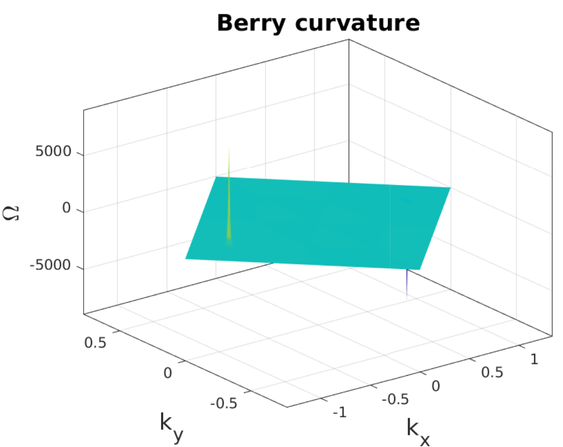
Fig. 6.2.1 Berry curvature of the graphene-boron-nitride heterostructure.
In this section, we compute the Berry curvature of the first conduction
band of the graphene-boron-nitride heterostructure. Let’s define the
input file gbn_lcao_scf.input as follows
LCAO.status = 1
info.calculationType = 'self-consistent'
info.savepath = './results/gbn_lcao_scf'
atom.element = [1 1 2 3]
da = 3.0425
atom.fracxyz = [2/3 1/3 0.5 + da/30
1/3 2/3 0.5 + da/30
2/3 1/3 0.5 - da/30
1/3 2/3 0.5 - da/30]
la = 4.648725932
domain.latvec = [[1/2  sqrt(3)/2     0]*la
[1/2 -sqrt(3)/2     0]*la
[0            0    30]]
domain.lowres = 0.3
element(1).species = 'C'
element(1).path = './C_ONCV_LDA.mat'
element(2).species = 'B'
element(2).path = './B_ONCV_LDA.mat'
element(3).species = 'N'
element(3).path = './N_ONCV_LDA.mat'
kpoint.gridn = [15,15,1]
This is a standard self-consistent calculation input file which will
provide us with the ground state density (and Hamiltonian). You may
execute the program typing
rescu -i gbn_lcao_scf.input
Next, we define the input file gbn_lcao_ber.input
info.calculationType = 'berry-curvature'
info.savepath = './results/gbn_lcao_ber'
rho.in = './results/gbn_lcao_scf'
kpoint.gridn = [102,102,1]
berry.bandIndex = 9
Here are the key elements:
RESCU find the eigenvalues and eigenstates on a two-dimensional Monkhorst-Pack grid and then computes the Berry curvature when set to
berry-curvature;Points RESCU to the ground state results;
Defines the size of the Monkhorst-Pack grid. The Berry curvature typically requires very high k-sampling, here we use more than \(10^{4}\) k-points. Alternatively, one can define a custom k-point mesh using the keyword
kpoint.kdirect(seeinputDescription.mfor more details);Determines the band index for which the Berry curvature is calculated (see Eq. (6.1.3)).
You may then run the program as follows
rescu -i gbn_lcao_ber
Upon return, the results will be in ./results/gbn_lcao_ber.mat. One
may find the Berry curvature in the structure component berry.Omega.
The Berry curvature can also be visualize typing
rescu -p results/gbn_lcao_ber
The resulting graph should look like the one in Fig. 6.2.1.
Chen Hu, Vincent Michaud-Rioux, Wang Yao, and Hong Guo. Moiré Valleytronics: Realizing Dense Arrays of Topological Helical Channels. Physical Review Letters 121.18 (2018), p. 186403.
Chen Hu, Vincent Michaud-Rioux, Wang Yao, and Hong Guo. Theoretical Design of Topological Heteronanotubes. In: Nano Letters 19.6 (June 2019), pp. 4146–4150.
Xinjie Wang, Jonathan R. Yates, Ivo Souza, and David Vanderbilt. Ab initio calculation of the anomalous Hall conductivity by Wannier interpolation.. Phys. Rev. B 74 (19 Nov. 2006), p. 195118.