15. Phonon calculation (finite displacement)
RESCU can perform phonon computations using the finite-displacement method [PLK]. The workflow of a phonon computation goes as follows. Firstly, RESCU extends the structure to a designated supercell structure. Then it determines its symmetries, generates non-equivalent displacements and carries out a self-consistent calculation for every atomic configuration. Input/output files are generated for each non-equivalent displacement such that the self-consistent calculations can be executed in parallel. Upon completion, the output files contain the Hellmann-Feynman forces experienced by each atom. Finally, RESCU calculates the force constants, dynamical matrices and related quantities such as the phonon band structure. In this section, we present the example of a bulk fcc silicon.
Note
Run each phonon calculation example in a separate directory.
RESCU creates intermediate result files such as disp.dat,
FORCE_SETS, and FORCE_CONSTANTS. These files are automatically
reused if they already exist in the working directory. If you run multiple
phonon examples (e.g., for different materials or calculation modes) in
the same folder, RESCU may unintentionally skip some steps by reading
results from a previous run. This can lead to incorrect or incomplete
calculations.
To avoid conflicts and ensure accurate results, create a clean folder for each example. This isolates the generated files and prevents RESCU from using outdated or incompatible data.
15.1. Example: silicon
Let’s create the file si_real_phonon.input as follows.
info.savepath = './results/si_real_phonon'
info.calculationType = 'phonon'
atom.element = ones(2,1)
atom.xyz = 10.25*[0 0 0;0.25 0.25 0.25]
domain.latvec=10.25/2*[0 1 1;1 0 1;1 1 0]
domain.lowres = 0.4
element(1).species = 'Si'
element(1).path = './Si_TM_LDA.mat'
functional.list = {'XC_LDA_X','XC_LDA_C_PW'}
kpoint.gridn = [3,3,3]
ph.mode = 'phonon'
ph.dr = 0.2
ph.supercellDimension = [2 2 2]
ph.ASR = 1
ph.qpointSympoints = {{[0,0,0] 0.5*[1,0,1]} {0.5*[2,1,1] [0,0,0]} {[0,0,0] 0.5*[1,1,1]}}
ph.labels = {'G','X','X1','G','G','L'}
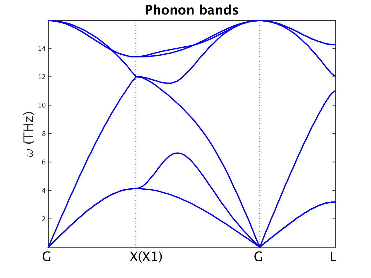
Fig. 15.1.1 Phonon band structure of fcc silicon
The meaning of the phonon parameters (ph.xxx) is described below.
info.calculationTypeis set to phonon so that RESCU performs a phonon calculationph.modeis a string that determines which step of a phonon calculation is to be done. You will most often use thedisplacement,phononandpostmodes. There are eight options:bands: RESCU reads the FORCE_CONSTANTS file, constructs the effective dynamical matrix and computes the phonon frequencies along the designated k-point line.displacement: RESCU determines the non-equivalent displacements and prints out input and XYZ files for each of them.gamma: is of boolean type. When it is true, the supercell size is automatically 1\(\times\)1\(\times\)1. This is used to obtain exact phonon frequencies at the \(\Gamma\)-point only.forcesets: RESCU combines the atomic forces stored in the files FORCESN (\(N=1,...,N_{disp}\)) into a single file: FORCE_SETS.forceconstants: RESCU uses the FORCE_SETS file together with symmetry operations to calculate the force constants of the supercell structure, and then stores the results in a file FORCE_CONSTANTS.phonon: RESCU performs all calculations necessary to obtain a phonon band structure:symmetry,``displacement``,``self-consistent``,``forcesets``,``forceconstants`` andbands.post: RESCU uses the self-consistent results`` forces to perform the following calculations:forcesets,``forceconstants``, andbands.symmetry: RESCU analyzes the structure and gives information about the number of symmetrical operations.
ph.drdetermines the magnitude of the atomic displacements in Bohr. A typical value is around 0.1 Bohr. It is advisable to take dr to be the same order as domain.lowres to mitigate the eggbox effect.ph.supercellDimensionis a most important parameter which determines the size of the supercells used to calculate the interatomic force constants. Large supercells generally yield better results, but demand more computational resources.ph.ASRswitch for the Acoustic-Sum-Rule (ASR) correction scheme. If ph.ASR is true, the ASR is enforced. Theoretically, the \(\Gamma\)-point of a 3D bulk system should have 3 zero frequencies, which are part of the so-called acoustic phonon branches. The ASR correction scheme usually improves the accuracy at the \(\Gamma\)-point.ph.qpointSympointsis a cell array of high symmetry point symbols or row-vectors in fractional coordinates that gives the path of k-points when calculating phonon band structures. One may write, for instance, ph.qpointSympoints={\(k_0\) \(k_1\) … \(k_n\)}, where tuples are typically are high-symmetry points of the first Brillouin zone. Here we define three such lines which are all contained in a cell array.ph.labelsis a cell array of strings labeling the k-points {\(k_0\) \(k_1\) … \(k_n\)} given inph.qpointSympoints. The labels will show on the phonon band structure plot.ph.qpointGridn(not used in example) is an integer that determines the number of k-points along the line given byph.qpointSympoints.ph.plot(not used in example) is of boolean type and it tells RESCU whether to plot the phonon band structure and save it as a .png file.
You may perform the calculation typing
rescu -i si_real_phonon.input
Upon completion, the following files have been produced: disp.dat, FORCE_SETS and FORCE_CONSTANTS. Their units are Å, eV/Å and eV/Å\(^2\), respectively. The phonon band structure of silicon is shown in Fig. 15.1.1.
15.2. Example: black phosphorus
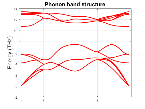
Fig. 15.2.1 Phonon band structure of a black phosphorus monolayer.
In section 1.1, we show how the phonon mode of
phonon calculations computes the phonon band structure of a material in
one shot. It is often impractical or inefficient to use the phonon
mode for research activities. In this section, we thus show how to
perform a phonon band structure calculation step-by-step using black
phosphorus as an example. First, create the following input file under
the name bp_real_disp.input.
info.calculationType = 'phonon'
info.savepath = 'results/bp_real_disp'
atom.element = ones(4,1)
atom.xyz = [0.0 0.053831313 4.704675810
1.660810589 1.549175746 4.704675810
1.660810589 2.343841383 2.572460227
0.0 3.839185675 2.572460227]
domain.latvec = [3.3216214769 0.0 0.0
0.0 4.5800202998 0.0
0.0 0.0 10.0]
domain.lowres = 0.4
units.length = 'a'
element(1).species = 'P'
element(1).path = './P_TM_LDA.mat'
ph.supercellDimension = [4 4 1]
ph.dr = 0.4
ph.mode = 'displacement'
Then execute it as follows
rescu -i bp_real_disp.input
The structure of black phosphorus is such that there are four
non-equivalent displacements. RESCU thus creates four input files,
1displaced.input, 2displaced.input, 3displaced.input and
4displaced.input and four corresponding XYZ files containing the
atomic coordinates and magnetic moments. For example,
1displaced.input looks as follows:
domain.lowres = 0.4
units.length = 'a'
element(1).species = 'P'
element(1).path = './P_TM_LDA.mat'
kpoint.gridn = [1,1,1]
mixing.tol = [1e-6,1e-6]
info.calculationType = 'self-consistent'
info.savepath = 'results/1displaced'
domain.latvec = [+1.32864859076e+01 0.0 0.0
0.0 +1.83200811992e+01 0.0
0.0 0.0 10.0]
atom.xyz = '1displaced.xyz'
atom.magmom = '1displaced.xyz'
atom.nvalence = 320
units.latvec = 'a'
units.xyz = 'a'
RESCU reproduces the phonon calculation input file at the exception of a
few parameters. Firstly, info.calculationType is changed to
self-consistent to compute the atomic forces and info.savepath
is set to a displacement-dependent name to avoid overwriting other
results. Next, the lattice vectors domain.latvec, atomic coordinates
atom.xyz, magnetic moments atom.magmom and total valence charge
atom.nvalence are changed to their supercell counterparts. Finally,
units.latvec and units.xyz are set to angstroms since the phonon
calculator interface employs those units.
One may then modify the self-consistent input files as he sees fit and proceed with the self-consistent calculations.
rescu -i 1displaced.input
rescu -i 2displaced.input
rescu -i 3displaced.input
rescu -i 4displaced.input
Note that these calculations can be submitted independently on a
cluster. After completing all calculations, the forces are saved in
results/xdisplaced.mat.
Finally, we obtain the band structure of black phosphorus by performing
a phonon calculation in post mode (which stands for
post-calculation). As mentioned in section 1.1, the
post mode reads the supercell forces, computes the force sets, force
constants, dynamical matrix and band structure. In the present exercice,
this is achieved creating the file bp_real_post.input as follows.
info.calculationType = 'phonon'
info.savepath = 'results/bp_real_post'
atom.element = ones(4,1)
atom.xyz = [0.0 0.053831313 4.704675810
1.660810589 1.549175746 4.704675810
1.660810589 2.343841383 2.572460227
0.0 3.839185675 2.572460227]
domain.latvec = [3.3216214769 0.0 0.0
0.0 4.5800202998 0.0
0.0 0.0 10.0]
domain.lowres = 0.4
units.length = 'a'
element(1).species = 'P'
element(1).path = './P_TM_LDA.mat'
ph.supercellDimension = [4 4 1]
ph.dr = 0.4
ph.mode = 'post'
ph.qpointSympoints = {[0 0 0] [0 1/2 0] [1/2 1/2 0] [1/2 0 0] [0 0 0]}
ph.labels = {'G','Y','M','X','G'}
ph.plot = true
The file looks just like bp_real_disp.input, but we have defined the
k-point line via the keywords ph.qpointSympoints and ph.labels.
We also set ph.plot to true to force RESCU to display the band
structure after computing it. The band structure is shown in
Fig. 15.2.1.
Parlinski, K., Z. Q. Li, and Y. Kawazoe. First-principles determination of the soft mode in cubic ZrO 2. Physical Review Letters 78.21 (1997): 4063.