18.1. Collinear spin
The ability to account for spin is crucial in simulating many systems. The most basic version of spin-dependent DFT calculation is collinear spin DFT. In collinear spin DFT, the spin-up and spin-down components are only coupled through the Hartree equation and exchange-correlation functional. It follows that the the Kohn-Sham Hamiltonian for the spin-up and spin-down wavefunctions can be diagonalized independently in a given self-consistent step. This alleviates the computational burden of diagonalization in addition to accelerating overall convergence due to constraint on spin directions. In this section, we show how to perform collinear spin calculation using the example of iron.
18.2. Example: iron
Here is the input file for the self-consistent calculation. In this example, we let RESCU decide of the physical parameters based on the pseudo-potential file Fe_TM_LDA.mat. It will use the most accurate parameters by default. In the present case, this means Kleinmann-Bylander projectors up to \(L=3\) and a double-zeta polarized atomic orbital basis to initialize the subspace. Iron adopts a perfect body-centered cubic geometry. We use the LDA for a DFT and use fast Fourier transforms for differentiation. The computation is rather costly since the pseudo-potential is hard, and hence it requires a higher resolution then says silicon, the complexity of its bands requires a fine Monkhorst-Pack grid and there is an additional spin components. To reduce the computational cost, we use all available symmetries setting symmetry.spacesymmetry to true. Finally, we use the tetrahedron method with Blöchl correction to compute the electron populations.
info.calculationType = 'self-consistent'
info.savepath = 'results/fe_real_collin_scf';
element(1).species = 'Fe';
element(1).path = './Fe_TM_LDA.mat';
atom.xyz = [0 0 0];
atom.element = 1;
atom.magmom = 3;
domain.latvec = (ones(3)-2*eye(3))/2*5.332428795; % define atoms positions in angstrom
domain.lowres = 1/4;
functional.list = {'XC_LDA_X','XC_LDA_C_PW'};
mixing.type = 'density';
kpoint.gridn = [9,9,9];
kpoint.sampling = 'tetrahedron+blochl';
spin.type = 'collinear';
We describe the spin keywords below.
atom.magmomthis is the magnetization, in unit of Bohr magneton, of the initial density;spin.typedetermines the spin description. The allowed values are degenerate, collinear and non-collinear. Degenerate is the default value and non-collinear will be discussed in another section.
By inspecting the output file, we can calculate a magnetic moment of 2.189 Bohr magnetons. The band structure is shown in Fig. 18.2.1. A splitting of roughly 2 eV is apparent, which is what we expect from the magnetic moment. Finally, we mention that this calculation could have been done using atomic orbitals just as well.
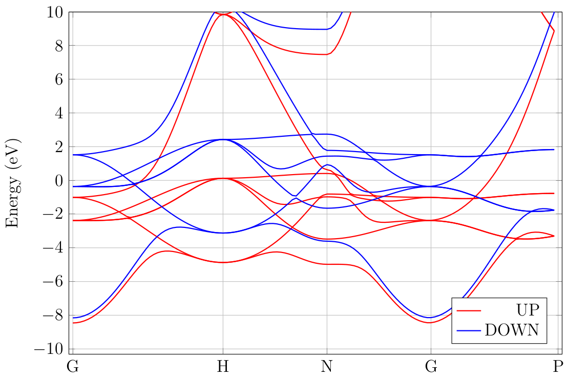
Fig. 18.2.1 Band structure of BCC iron