Accuracy parameter convergence tutorial

Requirements

Software components

• nanotools

• RESCU+

Pseudopotentials

I will need the following pseudopotential file.

• C_AtomicData.mat

Let’s copy it from the pseudo database to the current working directory and export RESCUPLUS_PSEUDO=$PWD.

Briefing

In this tutorial, I show how to converge the resolution for a diamond calculation.

Code

from nanotools import Atoms, Cell, System, TotalEnergy
from nanotools.checkconv import CheckPrecision
a = 3.562 / 2.
cell = Cell(avec=[[0.,a,a],[a,0.,a],[a,a,0.]], resolution=0.20)
fxyz = [[0.00,0.00,0.00],[0.25,0.25,0.25]]
atoms = Atoms(fractional_positions=fxyz, formula="CC")
sys = System(cell=cell, atoms=atoms)
ecalc = TotalEnergy(sys)
ecalc.solver.set_stdout("resculog.out")
calc = CheckPrecision(ecalc, parameter="resolution", etol=1.e-3)
calc.solve()
fig = calc.plot()

Explanations

CheckPrecision calculators are used to verify convergence of the total energy of a system with respect to precision parameters. In general, one should validate the precision of the grid resolution cell.resolution and k-sampling (in crystals) kpoint.grid. Here is a high level view of the calculation workflow:

1. Create a TotalEnergy calculator and specify calculation parameters like resolution, k-sampling, tolerance, etc.

2. Create a CheckPrecision calculator choosing a parameter to monitor the total energy tolerance.

3. Solve the Kohn-Sham equation varying the accuracy parameter until reaching the total energy threshold.

Total energy calculator

I first define a diamond crystal system with a lattice constant of 3.562 Ang. I set the resolution to a rather coarse value 0.2 Ang. I then create a total energy calculator (ecalc) from this System object. Here I set

solver.set_stdout("resculog.out")

which will redirect the output of all calculations to resculog.out. For more detail on how to setup a total energy calculation, refer to total energy tutorial.

CheckPrecision calculator

I can then initialize a CheckPrecision calculator from the total energy calculator and call solve. I set parameter to resolution since I want to determine the converged resolution (the alternative is k-sampling). I also set the total energy tolerance (per atom) etol to 1 meV. The solve function performs a series of calculations gradually decreasing the value of cell.resolution. The result of the first computation are saved to nano_scf_out_0.json, the second to nano_scf_out_1.json and so on. The total energy difference between two subsequent calculations is displayed on screen as follows

    resolution (ang) |    total energy (ev) |    delta energy (ev)
          0.20000000 |        -327.78347460 |        -327.78347460
          0.18000000 |        -327.78027295 |          +0.00320164
          0.16200000 |        -327.78410392 |          -0.00383096
          0.14580000 |        -327.78001823 |          +0.00408569
          0.13122000 |        -327.78244174 |          -0.00242351
          0.11809800 |        -327.78039611 |          +0.00204563
          0.10628820 |        -327.78158076 |          -0.00118465
          0.09565938 |        -327.78156284 |          +0.00001792

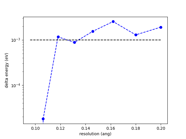
The procedure stops when delta energy falls below the attribute etol. The calculator will save results to nano_check_resolution.json as the solving progresses. The results can then be loaded with the class method read. On exit, the total energy differences are recalculated with respect to the smallest resolution value and shown on screen

    resolution (ang) |    total energy (ev) |    energy error (ev)
          0.20000000 |        -327.78347460 |          -0.00191175
          0.18000000 |        -327.78027295 |          +0.00128989
          0.16200000 |        -327.78410392 |          -0.00254108
          0.14580000 |        -327.78001823 |          +0.00154461
          0.13122000 |        -327.78244174 |          -0.00087890
          0.11809800 |        -327.78039611 |          +0.00116673
          0.10628820 |        -327.78158076 |          -0.00001792
          0.09565938 |        -327.78156284 |          +0.00000000

One could then decide that, say, 0.145 Ang is close enough to etol instead of the converged value of 0.106 Ang. You can finally see the total energy error as a function of resolution typing

fig = calc.plot()

which will produce