Dielectric constant (via finite-field) tutorial

Requirements

Software components

• nanotools

• RESCU+

Pseudopotentials

I will need the following pseudopotential file:

• C_LDA_TM_DZP.mat

Let’s copy it from the pseudo database to the current working directory and export RESCUPLUS_PSEUDO=$PWD.

Briefing

In this tutorial, I show how to calculate the dielectric constant of diamond looking at the screening of a finite external potential.

Code

An xyz file named diamond.fxyz

8
# diamond
C   0.0000   0.0000   0.0000
C   0.0000   0.5000   0.5000
C   0.5000   0.0000   0.5000
C   0.5000   0.5000   0.0000
C   0.2500   0.2500   0.2500
C   0.2500   0.7500   0.7500
C   0.7500   0.2500   0.7500
C   0.7500   0.7500   0.2500

and the following Python script

from nanotools import Atoms, Cell, System, TotalEnergy
from nanotools.dielectric import DielectricConstant
a = 3.562
cell = Cell(avec=[[a,0.,0.],[0.,a,0.],[0.,0.,a]], resolution=0.15)
atoms = Atoms(fractional_positions="diamond.fxyz")
sys = System(cell=cell, atoms=atoms)
sys.supercell([4,1,1])
ecalc = TotalEnergy(sys)
ecalc.solver.set_mpi_command("mpiexec -n 16")
calc = DielectricConstant(ecalc, axis=0, amplitude=0.1)
calc.solve()
die = calc.get_dielectric_constant()
print(f"epsilon = {die}")
fig = calc.plot_external_potential()

Explanations

In this section, I show how to obtain the dielectric constant of diamond. Here is a high level view of the calculation workflow:

1. Create a TotalEnergy calculator and specify calculation parameters like resolution, k-sampling, tolerance, etc.

2. Create a DielectricConstant calculator.

3. Solve the Kohn-Sham equation for a system in vacuum and a system in a finite external potential and compute the dielectric constant.

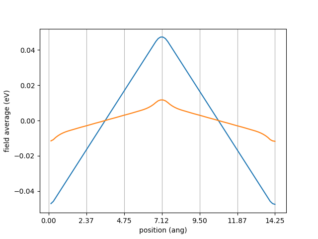
I will introduce a sawtooth potential which preserve periodic boundary conditions. The electrons will react by screening the external potential. The difference between the vacuum system and biased system will be a sawtooth potential scaled by the dielectric constant. In other words, I will compute

\[\epsilon = {\partial V^{saw}(\mathbf{r}) \over \partial\mathbf{r}} / {\partial \Delta V^{eff}(\mathbf{r}) \over \partial\mathbf{r}}\]

where the derivatives are taken at the center of the linear sections of the sawtooth potential.

Total energy calculator

I first define a diamond crystal system with a lattice constant of 3.562 Ang. I create a \(4\times 1\times 1\) supercell because I want the sawtooth potential to be linear over a relatively extended region. It is good practice to test various supercell lengths. I then create a total energy calculator (ecalc) from this System object. For more detail on how to setup a total energy calculation, refer to total energy tutorial.

Dielectric constant calculator

I then initialize a DC calculator from the total energy calculator. I also specify the parameters axis and amplitude which control along which axis the sawtooth potential varies and what is the amplitude of the sawtooth potential. The amplitude should not be too large, otherwise the linear response approximation will break down, and not too small, otherwise numerical inaccuracies will creep in. The left and right fit should give the same answer, as they do here. Asymmetry may arise if the sawtooth potential does not break on atomic plane. The vacuum and perturbed systems are solved invoking solve. The calculator will save results to nano_die_out.json as the solving progresses. The results can then be loaded with the class method read.

The value of the dielectric constant can be calculated calling

die = calc.get_dielectric_constant()
print(f"epsilon = {die}")

yielding epsilon = 5.578101320105986.

The linear response approximation is verified plotting \(V^{saw}(\mathbf{r})\) and \(\Delta V^{eff}(\mathbf{r})\). Calling plot_external_potential you should see