ASE tutorial
Requirements
Software components
ASE
nanotools
RESCU+
Pseudopotentials
I will need the following pseudopotentials.
Si_AtomicData.mat
Let’s copy them from the pseudo database to the current working directory and export RESCUPLUS_PSEUDO=$PWD.
References
Briefing
In this tutorial, I explain how to find the equilibrium positions of the atoms of a silicon unit cell using ASE.
Code
from ase.build import bulk
from ase.optimize import BFGS
from nanotools.ext.calculators.ase import Rescuplus
import os

nprc = 20
a = 5.43  # lattice constant in ang
atoms = bulk("Si", "diamond", a=a)
atoms.rattle(stdev=0.05, seed=1)  # move atoms around a bit
# rescuplus calculator
# Nanobase PP Si_AtomicData.mat should be found on path RESCUPLUS_PSEUDO (env variable)
inp = {"system": {"cell": {"resolution": 0.16}, "kpoint": {"grid": [5, 5, 5]}}}
inp["energy"] = {"forces_return": True, "stress_return": True}
inp["solver"] = {
    "mix": {"alpha": 0.5},
    "restart": {"DMRPath": "nano_scf_out.h5"},
    "mpidist": {"kptprc": nprc},
}
cmd = f"mpiexec -n {nprc} rescuplus -i PREFIX.rsi > resculog.out && cp nano_scf_out.json PREFIX.rso"
atoms.calc = Rescuplus(command=cmd, input_data=inp)
# relaxation calculation
os.system("rm -f nano_scf_out.h5")
opt = BFGS(atoms, trajectory="si2.traj", logfile="relax.out")
opt.run(fmax=0.01)
Explanations
Here is a high level view of the calculation work flow:
Build the system using ASE.
Create a calculator and link it to an
Atomsobject.Relax the structure using RESCU+ as a force calculator and ASE as an optimization engine.
Use ASE to read and analyse the results.
Build the system
Let’s first load some Python modules and class definitions.
from ase.build import bulk
from ase.optimize import BFGS
from nanotools.ase.calculators.rescuplus import Rescuplus
import os
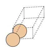
I build a silicon primitive cell with lattice parameter of 5.43 Ang as follows.
a = 5.43 # lattice constant in ang
atoms = bulk("Si", "diamond", a=a)
atoms.rattle(stdev=0.05, seed=1) # move atoms around a bit
# view(atoms)
I used the bulk function imported from the module ase.build.
This function is quite handy to build various basic crystals.
I note in passing the existence of the orthorhombic and cubic options, which allow building non-primitive cells.
The bulk function returns an Atoms object which essentially consists in attributes and methods describing a collection of atoms in a unit cell.
For instance, I can access the positions directly reading the attribute atoms.positions.
The Atoms class has a method rattle which moves the atoms in random directions.
Since I will show how to relax the atomic positions, I use rattle to move the atoms away from their equilibrium positions.
Finally, one may visualize the resulting lattice and atoms using the function view from the ase.visualize module.
Create a rescuplus calculator
The following step is creating and linking a Rescuplus calculator.
If you haven’t done so already, you should go through the total energy tutorial tutorial_etot.md.
Next, proceed as follows.
# rescuplus calculator
# Nanobase PP Si_AtomicData.mat should be found on path RESCUPLUS_PSEUDO (env variable)
inp = {"system": {"cell": {"resolution": 0.16}, "kpoint": {"grid": [5, 5, 5]}}}
inp["energy"] = {"forces_return": True, "stress_return": True}
inp["solver"] = {
    "mix": {"alpha": 0.5},
    "restart": {"DMRPath": "nano_scf_out.h5"},
    "mpidist": {"kptprc": nprc},
}
cmd = f"mpiexec -n {nprc} rescuplus -i PREFIX.rsi > resculog.out && cp nano_scf_out.json PREFIX.rso"
atoms.calc = Rescuplus(command=cmd, input_data=inp)
I first define a command including the MPI launcher to invoke the relevant program.
Here I will launch 20 MPI processes and call rescuplus which is the binary that compute the ground state density and optionally the atomic forces.
ASE uses a tag PREFIX to recognize input and output files.
rescuplus must take in a file called PREFIX.rsi and ASE will expect a file called PREFIX.rso.
Since rescuplus produces an output nano_scf_out.json, I include
mv nano_scf_out.json PREFIX.rso
in the command definition.
Most simulation parameters are passed in a dictionary input_data.
Unlike the nanotools interface, the atoms’ species and positions need not be in the input_data dictionary since the information is already comprised in the Atoms object.
I still have to specify the following keywords:
system.cell.res: the grid resolution;system.kpoint.grid: the Brillouin zone grid;energy.forces_return: a switch for returning the forces (I need them in the relaxation procedure);solver.mix.alpha: mixing fraction;solver.restart.DMRPath: path to the real space density matrix (for restart).
I use the real space density matrix to restart the calculation from one atomic configuration to the next, because it accounts partially for the atoms’ displacements unlike the real space density.
RESCU+ will need valid Nanoacademic potential files (including atomic orbitals).
The pseudopotential files are specified in a list of dictionaries containing the label and path keys, defining a name and a pseudopotential for each species.
Here the list contains a single dictionary, for silicon.
Finally, the three ingredients are given to the Rescuplus calculator constructor and the resulting calculator object is put in atoms.calc.
I am now ready to compute the total energy and forces.
Relax the structure
The commands dealing with the relaxation are the following.
os.system("rm -f nano_scf_out.h5")
opt = BFGS(atoms, trajectory="si2.traj", logfile="relax.out")
opt.run(fmax=0.01)
To avoid initializing the calculation with a random density matrix, I use the os module to issue a command to delete nano_scf_out.h5.
I then use the BFGS class constructor to create an optimize object.
An optimize object is initialized by passing it an Atoms object.
Here, I also use the trajectory option to create a Trajectory file, which will record the atomic configuration of each optimization step.
I also use the logfile option to print the optimizer’s information to a file relax.out.
The output will look something like
      Step     Time          Energy         fmax
BFGS:    0 08:59:25     -215.084549        1.7785
BFGS:    1 08:59:27     -215.162876        1.3122
BFGS:    2 08:59:30     -215.249844        0.2989
BFGS:    3 08:59:32     -215.252701        0.1292
BFGS:    4 08:59:35     -215.253128        0.0745
BFGS:    5 08:59:38     -215.253336        0.0085
It allows me to keep track of the total energy (in eV) and the maximal force component (in eV/Ang) as the relaxation proceeds.
I may also import atomic configurations from si2.traj during or after the relaxation procedure as I will show in the next section.
Import the relaxed structure
Once the relaxation is over, I would like to import and analyze the structure.
This is done using the read function from the ase.io module.
The commands
from ase.io import read
atoms = read('si2.traj')
atoms.positions -= atoms.positions[0,:]
atoms.get_scaled_positions()
yield
array([[0.        , 0.        , 0.        ],
       [0.24991947, 0.24996223, 0.24999951]])
After using read to import the final Atoms object, I shift all atoms such that the first atom lies at the origin.
I then print the fractional coordinates calling the get_scaled_positions method of Atoms.
The results is quite close to the expected diamond crystal coordinates [0.,0.,0.] and [0.25,0.25,0.25].
More advanced tutorials are found on the ASE website.