AI-relaxer (CHGNet) tutorial
Requirements
Software components
nanotools
Briefing
Here comes the Artificial Intelligence-driven (AI) relaxer for general material systems! This guide will walk you through the process step by step.
In atomistic modeling and simulation, “relax” refers to the process of allowing the atoms or molecules of the system to adjust their positions and configurations in order to reach a state of minimal energy or equilibrium.
Why is it necessary to relax a material system before we do Density Functional Theory (DFT) or Molecular Dynamics (MD) simulations? Relaxing the atomistic structure before conducting DFT or MD simulations is crucial to ensure the system reaches an energetically favorable configuration. Initially, the atomic positions might be arbitrary or based on an initial guess, potentially leading to high-energy configurations. By allowing the structure to relax, the atoms adjust their positions to minimize the total energy of the system, achieving a more stable and physically realistic configuration. This relaxation process helps in obtaining accurate and reliable results from subsequent simulations, as it allows the system to settle into its equilibrium state, providing a better starting point for further analysis and exploration of the system’s properties.
Why use this relaxer when traditional DFT relaxation methods are available? While traditional DFT relaxation methods are powerful and reliable, they are also computationally expensive. Relaxations for systems with a few hundred to a few thousand atoms using traditional DFT can take anywhere from minutes to several hours or even days, depending on factors such as computational resources, software efficiency, system size, convergence criteria, chosen methodology, and the quality of initial guesses. To strike a balance between accuracy and efficiency, a method that is both fast and reasonably accurate is desired. CHGNet [1] is a pretrained universal neural network potential for charge-informed atomistic modeling, which is specifically designed to accurately predict atomic forces and energies for atomistic simulations. One can use CHGNet to relax a system with several hundreds or even thousands of atoms very efficiently, often in just a few minutes based on our tests.
The AI-relaxer facilitates the structure relaxation process using the Atomic Simulation Environment (ASE) [2] and the pretrained CHGNet force model. After relaxation, the relaxed atomic structure is saved for further use. One can also plot the total energy of the material system during the structural optimization and visualize the relaxation trajectory. The AI-relaxer significantly enhances the efficiency of material simulations.
Scripts
from nanotools.utils import ureg
from nanotools import AtomCell
from nanotools.relaxation.general_material import NBRelaxer

atoms = AtomCell(
    formula="Si8",
    fractional_positions=[[0.00, 0.00, 0.00],[0.00, 0.50, 0.50],[0.50, 0.00, 0.50],[0.50, 0.50, 0.00],
        [0.25, 0.25, 0.25],[0.25, 0.75, 0.75],[0.75, 0.25, 0.75],[0.8, 0.75, 0.25]]*ureg.dimensionless,
    avec=[[5.43, 0, 0], [0, 5.43, 0], [0, 0, 5.43]]*ureg.angstrom,
    pbc=[True, True, True]
    )

relaxer = NBRelaxer(atoms, relaxation_type="atom_partial_relax", fix_atoms_index=[1,7])
relaxer.relax()
relaxer.write(filename="Si8_relaxed")
relaxer.plot_energy(filename="Si8_relaxed")
relaxer.visualize_trajectory()
Explanations
This example demonstrates the relaxation for a Silicon system, providing the formula, the fractional positions, the lattice vectors, and the periodic boundary conditions flags.
In this script, we import the NBRelaxer class from the nanotools.relaxation.general_material module.
In this context, NB stands for “Nano Builder”. The NBRelaxer class is used to relax the material system using the CHGNet potential.
After importing the necessary modules, the first step is to create the material using the AtomCell object.
The positions parameter must be provided. If positions specifies the path of an xyz file, the formula parameter is automatically read from the xyz file.
Below is an example of reading data from a file path:
atoms = AtomCell(positions="PGY.xyz", avec=[[12.91068695, 0, 0], [10.44499195, 7.58867451, 0], [0, 0, 20.0]])
However, if positions does not specify an xyz file, formula must be used to define the chemical formula, as shown in the original example.
The avec parameter is used to define the lattice vectors. If the unit is not specified, the default unit is angstrom.
The pbc parameter is used to define the periodic boundary conditions. The default value is [True, True, True], which means the system is periodic in all three directions.
The next step involves creating the NBRelaxer object, which is used to relax the material system.
The NBRelaxer object takes the AtomCell objects of the material as inputs.
The relaxation_type parameter specifies the type of relaxation to be performed. Three relaxation types are supported:
“atom_partial_relax”, “cell_fractional_relax”, and “unconstrained_relax”.
“atom_partial_relax” relaxes the material while fixing certain atoms. The indices of the atoms to be fixed are specified using the fix_atoms_index parameter.
By default, the first atom is fixed.
The “cell_fractional_relax” type relaxes the unit cell while keeping the scaled positions fixed.
The “unconstrained_relax” type relaxes the material without fixing any atoms or unit cell parameters.
In this example, we use the “atom_partial_relax” type and fix the atoms at indices 1 and 7.
An example of the “cell_fractional_relax” type is shown below:
relaxer = NBRelaxer(atoms, relaxation_type="cell_fractional_relax")
The nanotools.relaxation.two_probe.relax() method initiates the relaxation process for the material.
relaxer = NBRelaxer(atoms, relaxation_type="atom_partial_relax", tolerance=0.01, max_steps=20)
Upon invocation, the nanotools.relaxation.two_probe.relax() method sets up the CHGNet calculator and initiates the relaxation process using the BFGS minimizer from the ASE package.
The relaxation process is terminated when the maximum number of steps is reached or the force on all atoms is below the specified tolerance.
By default, the force tolerance is set to 0.05 eV/angstrom, and the maximum number of steps is set to 100.
You can adjust these parameters by providing the tolerance and max_steps parameters, respectively.
The nanotools.relaxation.two_probe.write() method is used to write the relaxed structure to a file in a specified format.
It supports a variety of formats, including “vasp”, “xyz”, and “cif”, among others.
If no format is specified, the method defaults to exporting in the “xyz” format.
The filename parameter is optional. If it’s not provided, the method will use “relaxed”
as the default filename for the output file.
The nanotools.relaxation.two_probe.plot_energy() method is used to plot the potential energy during the optimization process and save it to a file.
You could decide whether to show the plot by setting the show parameter to True or False.
The filename parameter is optional. If it’s not provided, the method will use “Potential energy” as the default filename for the output file.
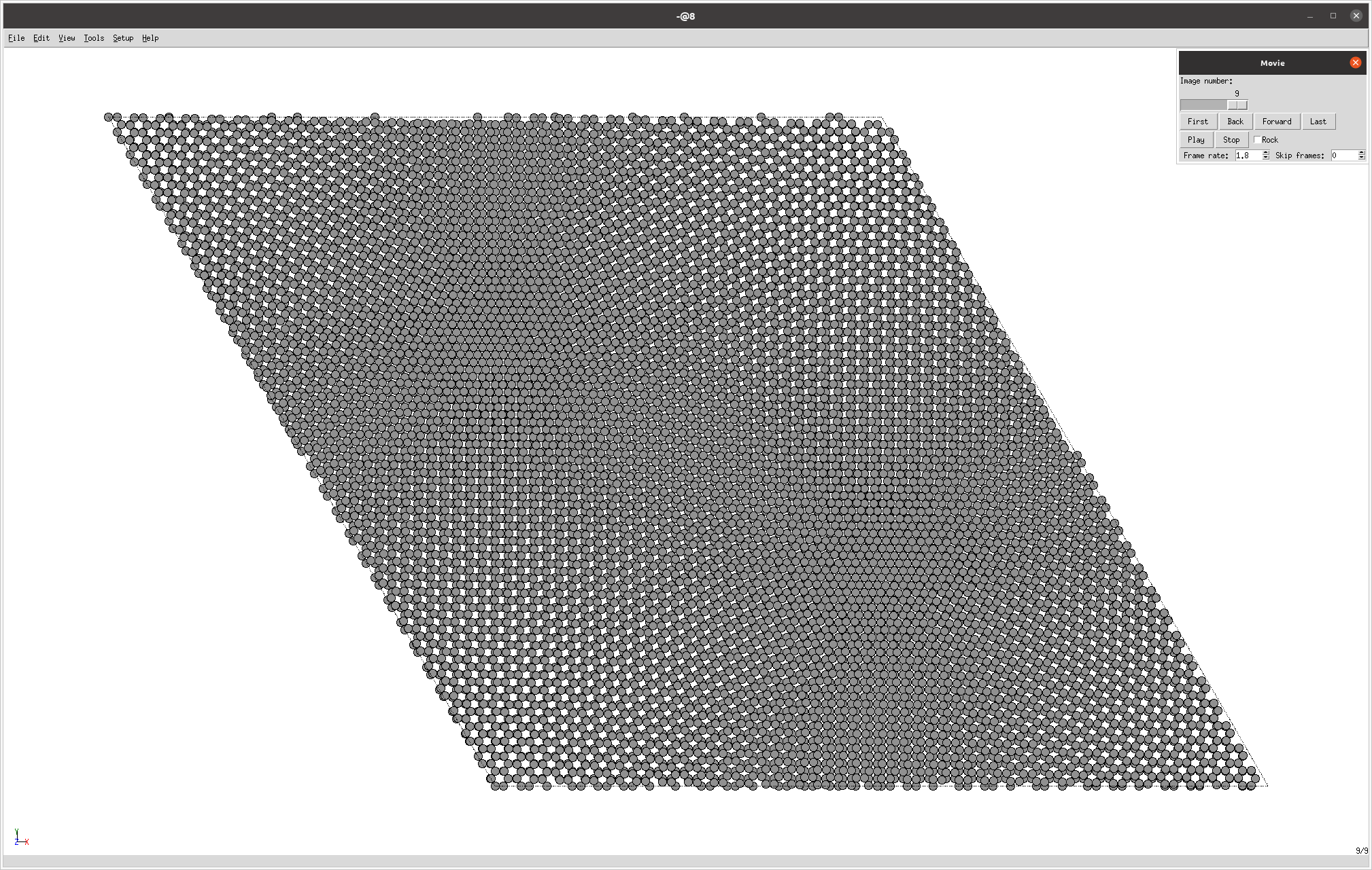
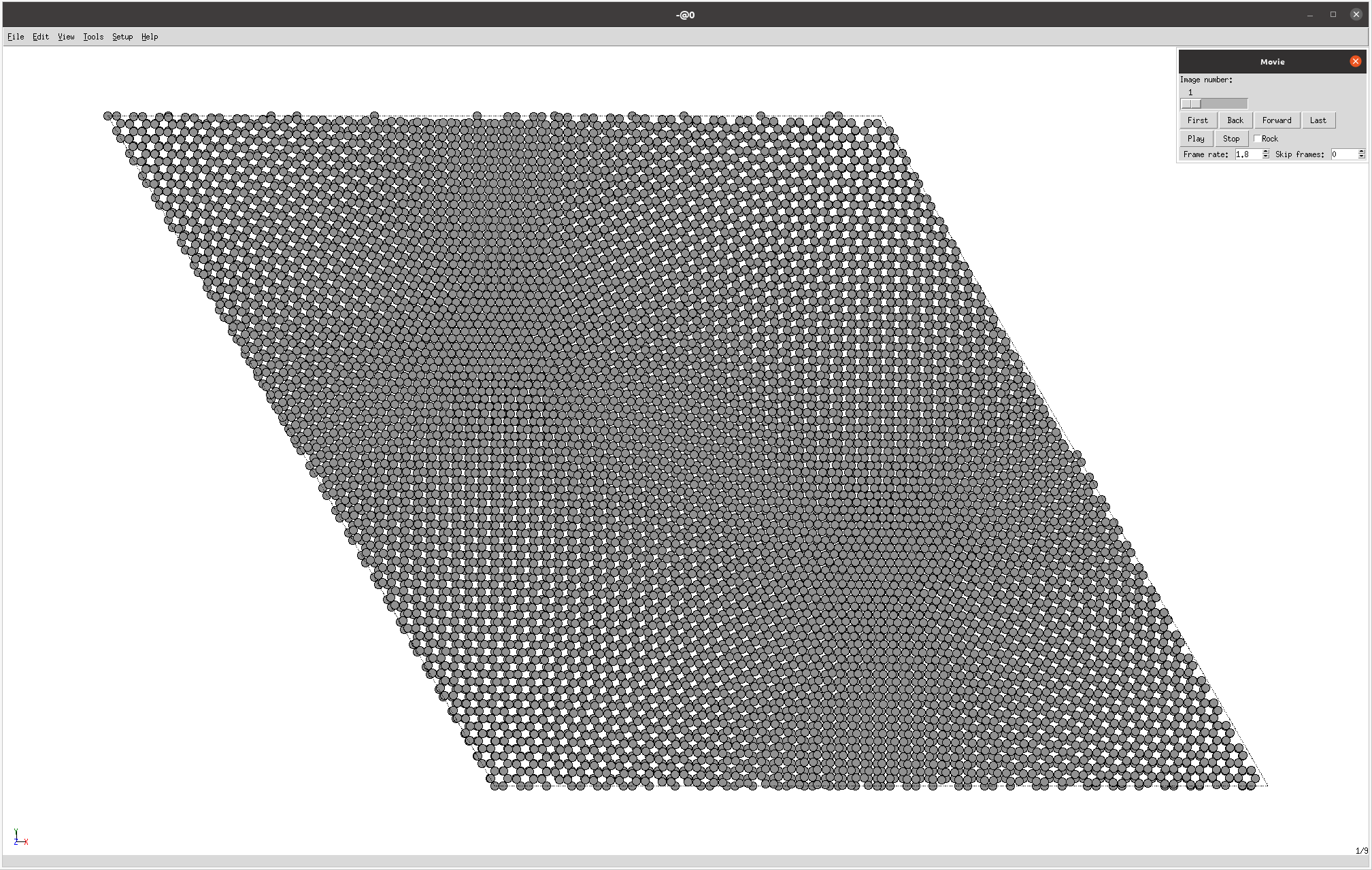
The nanotools.relaxation.two_probe.visualize_trajectory() method is used to visualize the trajectory of the relaxation process.
This method generates a series of images showing the atomic structure at different steps of the optimization process.
An example of the visualization of twisted bilayer graphene with 10,802 carbon atoms is shown below.
Before the relaxation:
After the relaxation (Due to the system’s size, atom position changes might not be apparent):