5. NanoDCAL support

Note

The tables below list the NanoDCAL calculations you can ask for. You request each one in plain language, and it runs on your own machine or on an HPC cluster. You can also build a transport project up over several requests. Results depend on the structure and settings you ask for, so review the generated decks and the outputs before you rely on them. Works with NanoDCAL 2022A and 3.1.1.

LatticeMind turns a plain-language request into a complete, launch-ready NanoDCAL workflow: it selects the calculation steps, builds the crystal or two-probe device structure, renders the input decks with a curated parameter vocabulary, stages the LCAO basis files with the project so it runs anywhere, executes the decks locally or on a remote server, and verifies the outputs before reporting results.

5.1. Configure NanoDCAL before the first run

Configure a valid LatticeMind license for startup; it activates LatticeMind whichever solver you select. To run NanoDCAL calculations, also configure:

1. A NanoDCAL executable, selected by LATTICEMIND_NANODCAL_CMD or the Web UI’s Local NanoDCAL command field.

2. A NanoDCAL license on the computer that runs the solver. Test a small NanoDCAL example directly before launching it through LatticeMind.

3. The extracted NeutralAtomDatabase from the Nanoacademic Portal, selected by LATTICEMIND_NANODCAL_DATA_PATH or the Web UI’s NanoDCAL neutral atom data field.

LatticeMind searches the configured database recursively, verifies that every requested element has a *.nad or *.mat file, and stages the selected files under the project’s nanodcal_basis/ directory. When sharing a project, please keep that directory within the scope of your Nanoacademic license. See Licenses and solver executables for complete local and remote setup.

5.2. Calculation types you can request

The prompts below have each produced a complete, verified run. Substitute your own material freely.

Ground state and energetics

Calculation	Example prompt	Key outputs
SCF	“Using NanoDCAL, run an SCF calculation for silicon.”	NanodcalObject.mat, total energy
Total energy	“Using NanoDCAL, calculate total energy for silicon.”	TotalEnergy.mat
Charge analysis	“Using NanoDCAL, calculate charge analysis for silicon.”	Charge.mat, per-atom charges
Effective potential	“Using NanoDCAL, calculate effective potential for silicon.”	EffectivePotential.mat
Electron density	“Using NanoDCAL, extract electron density for silicon.”	TotalElectronDensity.mat, integrated electron count
Starting fields	“Using NanoDCAL, create initialization, non-SCF rigid atomic field, and Harris-field decks for diamond germanium.”	initialization, non-SCF, and Harris-field objects
Combined ground-state properties	“Using NanoDCAL, calculate total energy, effective potential, electron density, and charge analysis for rocksalt MgO.”	all four property files after one SCF calculation

Electronic structure

Calculation	Example prompt	Key outputs
Band structure	“Using NanoDCAL, run an SCF and band-structure calculation for silicon.”	BandStructure.mat, band gap, plot
Full band structure	“Using NanoDCAL, run SCF and calculate full band structure for aluminum.”	FullBandStructure.mat
Complex band structure	“Using NanoDCAL, calculate the complex band structure for silicon.”	ComplexBandStructure.mat
Density of states	“Using NanoDCAL, calculate density of states for silicon.”	DensityOfStates.mat, plot
Joint DOS	“Using NanoDCAL, calculate the joint DOS for silicon.”	JointDensityOfStates.mat
Effective mass	“Using NanoDCAL, calculate the effective mass for GaAs.”	EffectiveMass.mat
Eigen-states and wavefunctions	“Using NanoDCAL, run SCF and calculate eigen-states, real-space wavefunction, and effective mass for silicon.”	EigenStates.mat, RealSpaceWavefunction.mat
Post-SCF and momentum	“Using NanoDCAL, run SCF, post-SCF spin-orbit coupling, and momentum analysis for silicon.”	CalculatedResults.mat, Momentum.mat
Spin polarization	“Using NanoDCAL, calculate spin polarization for ferromagnetic bcc iron.”	SpinPolarization.mat

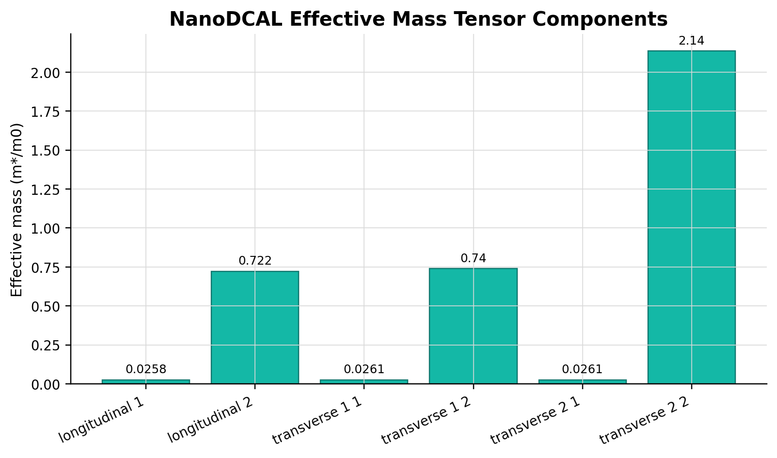
Fig. 5.2.1 Effective-mass tensor components for GaAs from the “calculate the effective mass for GaAs” prompt, as LatticeMind plots them from EffectiveMass.mat. The light longitudinal component and the heavier transverse ones are the conduction-band anisotropy the tensor separates.

Structure and mechanics

Calculation	Example prompt	Key outputs
Relaxation	“Using NanoDCAL, relax rocksalt MgO and calculate elastic modulus.”	relaxed structure
Forces and stress	“Using NanoDCAL, calculate the force and stress for silicon.”	Force.mat, Stress.mat
Elastic modulus	“Using NanoDCAL, relax diamond germanium and calculate force, stress, and elastic modulus.”	ElasticModulus.mat

Phonons (finite-displacement Hessian)

Calculation	Example prompt	Key outputs
Phonon band structure	“Using NanoDCAL, calculate the Hessian and phonon band structure for silicon.”	Hessian.mat, PhononBandStructure.mat
Phonon DOS	“Using NanoDCAL, calculate the Hessian and phonon density of states for silicon.”	PhononDensityOfStates.mat
Phonon full band structure	“Using NanoDCAL, calculate the Hessian, phonon band structure, and phonon full band structure for rocksalt MgO.”	PhononFullBandStructure.mat

Quantum transport (two-probe devices)

LatticeMind builds the full lead-SCF → device-SCF → property chain automatically from a one-line request.

Calculation	Example prompt	Key outputs
Transmission	“Using NanoDCAL, run a transmission calculation along z for a homogeneous aluminum two-probe device.”	Transmission.mat, T(E)
Conductance	“Using NanoDCAL, run a conductance calculation along z for a homogeneous aluminum two-probe device.”	ConductanceAndCurrent.mat
I–V curve	“Using NanoDCAL, run an I-V curve calculation along z for a homogeneous aluminum two-probe device.”	CurrentVoltageCurves.mat
Scattering states	“Using NanoDCAL, run a scattering-states calculation along z for a homogeneous aluminum two-probe device.”	ScatteringStates.mat
Transmission channels	“Using NanoDCAL, run SCF and transmission-channel analysis for ferromagnetic bcc iron.”	TransmissionChannel.mat
AC conductance and AC transmission	“Using NanoDCAL, run an AC conductance calculation along z for a homogeneous aluminum two-probe device.”	AcConductance.mat, AcTransmission.mat
Seebeck coefficient and thermoelectric current	“Using NanoDCAL, run a Seebeck coefficient calculation along z for a homogeneous copper two-probe device.”	SeebeckCoefficient.mat, ThermoelectricCurrent.mat — the transmission spectrum they integrate over is run first automatically
Photocurrent	“Using NanoDCAL, run a photocurrent calculation along z for a homogeneous aluminum two-probe device.”	Photocurrent.mat
Thermoelectric figure of merit ZT, phonon transmission channels	“Using NanoDCAL, calculate the Hessian and the thermoelectric figure of merit ZT along z for bulk copper.”	Hessian.mat, ThermoelectricProperties.mat, PhononTransmissionChannel.mat — the Hessian they consume is run first automatically

Devices are described in words. “A homogeneous aluminum two-probe device” builds the electrode from the bulk cell and the scattering region from that cell repeated along the transport axis; “an aluminum monatomic chain” builds a wire; supplied electrode and central-region structure files are used as given. A bias sweep such as “from 0 to 0.4 V in 0.2 V steps” becomes one biased device calculation per voltage feeding the I–V curve.

5.3. Continuing a transport project

A NanoDCAL project is a conversation. Each request below is a separate turn on the same project:

Using NanoDCAL, run a transmission calculation along z for a homogeneous
aluminum two-probe device.

Now compute the current-voltage curve for the same device from 0 to 0.4 V
in 0.2 V steps.

Looking only at this project's own outputs: what is the transmission at the
Fermi energy, and is it close to an integer channel count?

The second turn does not restate the device; it inherits it from the request the project was founded on, adds the biased device calculations and the I–V step, and reuses the converged electrode and device objects rather than recomputing them. The third turn changes nothing and answers from the project’s own results.

The same holds for adding a property — “Add a Seebeck coefficient calculation to this project, reusing everything it already has” inserts the transmission spectrum the Seebeck coefficient is integrated from and executes only what is new — and for standing policies: “From now on, every transmission calculation in this project must use energy points from -1 to 1 eV. Re-render the transmission deck accordingly.” re-renders the deck with the new window and keeps the device.

A long calculation can be released and collected later:

latticemind run "Using NanoDCAL, run a transmission calculation along z for a homogeneous aluminum two-probe device." \
    --solver nanodcal --execute --approve-execution --remote-profile cluster --detach

latticemind run --project <project-dir> \
    "Continue this project: collect the finished results and report the transmission at the Fermi energy." \
    --execute --approve-execution --remote-profile cluster

The first command returns as soon as the remote wave is running; the second reattaches to it, fetches what finished, and reports from it. See Releasing a long calculation.

5.4. Publish-ready figures and numeric summaries

After NanoDCAL writes a .mat result, LatticeMind reads the physical axes and units from that file and writes these project-local files:

• results/analysis_summary.json contains scalar and array-shape summaries, including the band gap, integrated electron count, transmission at the Fermi level, force maximum, stress maximum, and transport channel count when those quantities are present.

• figures/<name>.png is the 360 dpi report image embedded in report.html.

• figures/<name>.svg and figures/<name>.pdf are editable or vector exports for a manuscript.

• results/figure_manifest.json names the source .mat file and records every PNG, SVG, and PDF path, plus PNG dimensions and DPI.

The figure type follows the solver data:

• Band structures use Fermi-referenced energy axes. Effective-mass figures use electron/hole dispersion fits and directional components in units of \(m_e\).

• EigenStates.mat contains only the bands and k-points requested by calculation.eigenStates.numberOfBands and kSpaceGridNumber. For the silicon eigenstate prompt, [1,1] at a [1,1,1] grid selects one state below and one state above \(E_F\) at Γ. Their energy separation is a selected direct Γ-point separation, not the fundamental indirect band gap; request a band-structure calculation to determine the latter.

• EffectivePotential.mat and TotalElectronDensity.mat produce three orthogonal slices plus plane-averaged profiles.

• TransmissionChannel.mat produces transverse-k maps split by spin.

• Force, stress, and elastic-modulus figures use eV/Angstrom and GPa.

• NanodcalObject.mat, TotalEnergy.mat, and CalculatedResults.mat contribute descriptors but do not create a figure from saved-object or scalar-only arrays.

If one file contains an unsupported array shape, LatticeMind records the exact filename and parser error in results/analysis_summary.json.warnings and continues processing the other files. A follow-up request can regenerate the figures without rerunning NanoDCAL:

Reprocess the existing NanoDCAL outputs and regenerate all report figures
without rerunning the solver.

5.5. Execution options

• Local — runs against a local NanoDCAL installation. Local solver runs are serialized behind a machine-wide lock, so two LatticeMind sessions never start local calculations on top of each other; a run that has to wait says so.

• Remote — a profile in ~/.latticemind/remote_profiles.toml with the exact fields host, nanodcal_command, and shell_preamble. LatticeMind stages a self-contained bundle (decks, basis files, the converged objects and results a dependent deck reads, and the job script), runs it over SSH — or releases it with --detach to keep running after LatticeMind exits — and fetches the verified outputs back into the project. Multiple calculations can run in parallel on a multi-core server. See Remote & HPC execution.

• Portable basis — basis files travel with the project (nanodcal_basis/), so a project generated on one machine runs unchanged on another.

See also

For a worked NanoDCAL tutorial, see NanoDCAL: electronic structure and transport in the advanced tutorials.