4.1. Example: band structure of silicon
Firstly, we obtain the ground state density determining the Hamiltonian to be used in the band structure calculation.
info.calculationType = 'self-consistent'
info.savepath = './results/si_real_scf';
element(1).species = 'Si';
element(1).path = './Si_TM_PBE.mat';
atom.xyz = 10.25 * ...
   [[     0         0         0]
    [0.2500    0.2500    0.2500]];
atom.element = ones(2,1);
domain.latvec = 10.25/2*[0,1,1;1,0,1;1,1,0];
domain.lowres = 0.5;
diffop.method = 'fft';
functional.list = {'XC_GGA_X_PBE','XC_GGA_C_PBE'};
kpoint.gridn = [5,5,5];
The keywords are described below.
info.calculationTypeis a string determining the nature of the calculation. If it is set to self-consistent as it is here, the Kohn-Sham equation is solved self-consistently and the equilibrium ground-state density is saved upon completion of the calculation;info.savepathis a string containing the path to the results file. RESCU uses two files to save the data. One file is an HDF5 file which contains all the distributed arrays (e.g. density, kinetic energy density, wavefunctions) and the other file is a MAT-file which contains the rest of the results (e.g. total energy, Kohn-Sham energies, forces). In the present example, the files./results/si_real_scf.h5and./results/si_real_scf.matwill be created;element(1).speciesis a string containing the label of element(1);element(1).pathis a string containing the path to the pseudo-potential file associated with element(1);atom.xyzis an array containing the atom Cartesian coordinates;atom.elementis an array containing the element number associated with each atom. All eight atoms are element(1);domain.latvecis an array containing three lattice row vectors;domain.lowresis a number defining the grid resolution in Bohr radii;diffop.methodis a string determining the method used to compute derivatives. Fast Fourier transforms will be used here;functional.listcell array of strings containing the names of the functionals included in the DFT calculation; we use the PBE exchange correlation functional [PBE];kpoint.gridnuse a 5\(\times\)5\(\times\)5 uniform grid to sample reciprocal space.
RESCU is executed as follows
rescu -i si_real_scf
The next step is calculating the band structure. RESCU is notified to do
a band structure calculation through the keyword
info.calculationType. The path to the converged density is passed
using the keyword rho.in. Most of the self-consistent calculation
input should be reused as the system remains the same. Redundant data is
therefore read from rho.in. The output path must be modified,
otherwise the self-consistent results will be overwritten. Finally, the
kpoint keywords should also be different.
info.calculationType = 'band-structure'
info.savepath = './results/si_real_bs';
kpoint.type = 'line';
kpoint.gridn = 32;
kpoint.sympoints = {'L','G','X','W','K'};
rho.in = './results/si_real_scf';
The new keywords are described below.
info.calculationTypeis a string determining the nature of the calculation. If it is set to band-structure, the eigenvalues of the Hamiltonian are calculated. There is no self-consistent procedure involved;kpoint.typeis the string ’line’ which tells RESCU to compute a line going through the k-points defined by kpoint.sympoints and having a total of kpoint.gridn;kpoint.gridnuse 32 point along the line defined by kpoint.sympoints;kpoint.sympointscell array containing the reduced coordinates or conventional labels (FCC labels in the present example).rho.inthe path of the file containing the self-consistent density. Here we point to the result from the calculation done above.
For a band structure calculation, RESCU is executed as follows
rescu -i si_real_scf
Upon completion, RESCU will write the basic band structure data in
BandStructure.txt. The first three lines give the number of
high-symmetry k-points, their labels (e.g. \(L, \Gamma, X\) for an
FCC crystal) and their k-point indices. The next lines gives the total
number of k-points (\(n_k\), bands \(n_b\) and spin degrees of
freedom \(n_s\)). For example,
5                   # num high symmetry points
L G X W K           # label high symmetry points
1 21 44 55 63       # indices high symmetry points
63 10 1             # nk, nb, ns
Then comes the k-point fractional coordinates, i.e. a block of
\(n_k\) lines with three coordinates. Finally, there are the
energies, i.e. a block of \(n_k\) lines with \(n_b\) numbers. If
the simulation included spin, that last block is repeated twice.
Additional data is found in the band structure stored in
./results/si_real_bs.mat.
4.2. Band structure plot
Once the band structure calculation is over, the results can be read
directly from the output files. RESCU also has an automated plotting
option. Suppose that the results are stored in
./results/si_real_bs.mat, then they can be plotted typing
rescu -p ./results/si_real_bs.mat
This will read ./results/si_real_bs.mat, display a plot of the band
structure, and save the figure to si_real_bs_bs.fig. By default, the
figure is saved as a MATLAB figure and _bs is appended to the input
file’s name. It is also possible to determine the name and extension of
the output file as follows
rescu -p ./results/si_real_bs.mat EvsK_si.png
This would save the figure as a PNG file named EvsK_si.png. The
resulting figure should look like Fig. 4.2.1.
RESCU read the Fermi level off the input file and shift the energies
such that the Fermi level is zero. The k-point labels or coordinates
appear in the ordinate axis.
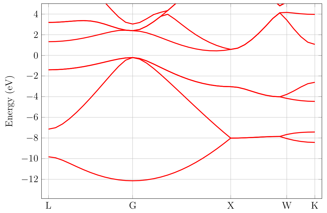
Fig. 4.2.1 Silicon band structure
Perdew, John P., Kieron Burke, and Matthias Ernzerhof. Generalized gradient approximation made simple (vol 77, pg 3865, 1996). Physical review letters 78.7 (1997): 1396-1396.