9.3. Example: LDOS of graphene
In this section, we show how to calculate a real space representation of
the DOS: the local density of states. LDOS calculations are quite
similar to DOS calculations, only that at the end, the density is
calculated only from states lying at a specific energy. Again, assuming
that the self-consistent ground state density of graphene may be found
in ./results/gr_lcao_scf.h5 and ./results/gr_lcao_scf.mat, one
may compute the LDOS of graphene using the following input script
info.calculationType = 'dos'
info.savepath = 'results/gr_lcao_ldos'
kpoint.sampling = 'tetrahedron'
kpoint.gridn = [45,45,1]
rho.in = 'results/gr_lcao_scf'
dos.ldos = true
We simply set the keyword dos.ldos equal to true. Let’s introduce a
few keywords providing additional control on the LDOS.
dos.ldosdetermines whether to calculate the local density of states.dos.ldosEnergycontains the energies at which the local density of states is calculated.dos.ldosERangethe LDOS will be calculated including all states within the range of energies given bydos.ldosERange(9.3.1). Notice that setting the value to \([-\infty,\epsilon_F]\) yields the ground state density.dos.ldosShiftEfif true, the LDOS energies are relative to the Fermi energy.
Note that the LDOS energies specified by dos.ldosEnergy or
dos.ldosERange are absolute unless the keyword dos.ldosShiftEf
is set to true. In the previous example, only dos.ldos is
specified, and hence the LDOS is calculated at the Fermi energy. The
LDOS is saved in the /dos/ldosVal data set of
./results/gr_lcao_ldos.h5. This is visible typing
h5disp('results/gr_lcao_ldos.h5')
Group '/dos'
Dataset 'ldosVal'
Size:  17152x1
MaxSize:  17152x1
Datatype:   H5T_IEEE_F64LE (double)
ChunkSize:  []
Filters:  none
FillValue:  0.000000
Attributes:
'real':  1.000000
As we have seen in the previous section, we expect the DOS to have \(p_z\) character there. This is indeed apparent in Fig. 9.3.1 which shows an isosurface of the LDOS.
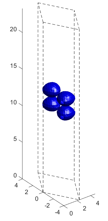
Fig. 9.3.1 LDOS of graphene at the Fermi level.
The projected LDOS (PLDOS) may also be calculated using the same
keywords as the projected DOS (see section 1.2). For
instance, you could set dos.projAtom = 1 in the above example and
you’d see a single \(p_z\) orbital instead of the two in
Fig. 9.3.1. The PLDOS are saved in the
/dos/pldosVal data set of ./results/gr_lcao_ldos.h5.