9.2. Example: PDOS of graphene
We now turn to partial density of states calculations and use graphene
to illustrate how to set them up. PDOS calculations are fundamentally
similar to DOS calculations, the difference being that the energy levels
constituting the DOS are weighted by atomic orbital coefficients.
Suppose that the self-consistent ground state density of graphene may be
found in ./results/gr_lcao_scf.h5 and ./results/gr_lcao_scf.mat,
one may compute the PDOS of graphene using the following input script
info.calculationType = 'dos'
info.savepath = 'results/gr_lcao_pdos'
kpoint.sampling = 'tetrahedron'
kpoint.gridn = [45,45,1]
rho.in = 'results/gr_lcao_scf'
dos.range = [-0.75,0.35]
dos.projL = [0,1,2]
dos.projM = -2:2
The relevant keywords in PDOS calculations are the following
dos.rangegives the energy range over which the DOS and PDOS are calculated. This is relative to the Fermi energy. The default units are Hartree.dos.projAtomis an array containing the atom indices on which to project the DOS.dos.projLis an array containing the orbital angular momenta on which to project the DOS.dos.projMis an array containing the projected orbital angular momenta on which to project the DOS.dos.projSpeciesis an array containing the species (element) indices on which to project the DOS.dos.projZis an array containing the \(\zeta\)-numbers on which to project the DOS.
It is not necessary to project the DOS onto all valid values of a given
quantum number. For instance, we could have set dos.projL equal to
[0,1]. Note however that the sum of the PDOS would not equal the DOS in
this case since part of the DOS has d-orbital character. Whereas the
values of dos.projAtom, dos.projL, dos.projSpecies and
dos.projZ are self-explanatory, dos.projM depends on the
convention for the real spherical harmonics used by RESCU, which may be
found in Table 2.8.1.
In the present example, we decompose the DOS using both dos.projL
and dos.projM. In this case, RESCU will decompose the DOS into all
valid – meaning that, say, dos.projL = 3 would be ignored since
there are no \(f\)-orbital in our atomic orbital basis –
combinations of the specified constraints. There are thus nine PDOS
calculated here. After loading the results, the dos data structure
should look like
       desc: [1x1 struct]
     dosvec: [1100x1 double]
     nrgvec: [1100x1 double]
    pdosdef: [9x5 double]
    pdosvec: [1100x1x9 double]
   projAtom: []
      projL: [0 1 2]
      projM: [-2 -1 0 1 2]
projSpecies: []
      projZ: []
In particular, the field dos.pdosdef contains the constraints
specific to each PDOS. The field dos.pdosdef has nine rows,
corresponding to the nine PDOS and five column corresponding to the
value of the atomic orbital indices. A negative value out of bound means
that the index is summed over. For instance, there is no minus-oneth
atom, so projAtom = -1 means that the contribution of all atoms is
accumulated. Similarly, projM = -4 means that the contribution of
\(Y_{l,m}\)-orbitals is summed over \(m\). In the latter case,
projM = -1 would simply refer to \(Y_{l,-1}\)-orbitals however.
dos.pdosdef
#projAtom projL projM projSpecies projZ
    -1     0     0    -1    -1
    -1     1    -1    -1    -1
    -1     1     0    -1    -1
    -1     1     1    -1    -1
    -1     2    -2    -1    -1
    -1     2    -1    -1    -1
    -1     2     0    -1    -1
    -1     2     1    -1    -1
    -1     2     2    -1    -1
The total DOS along with the \(s\), \(p_y\), \(p_z\) and
\(p_x\) PDOS (first four rows of dos.pdosdef respectively), are
plotted in Fig. 9.2.1. The low
lying state have \(s\) character while the Dirac cone is strictly
composed of \(p_z\) orbitals. The \(p_x\) and \(p_y\) PDOS
are virtually indistinguishable as expected from symmetry
considerations.
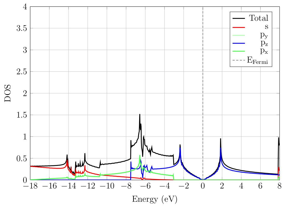
Fig. 9.2.1 PDOS of graphene.