23. Electron \(\mathbf{k} \cdot \mathbf{p}\) simulation of Jackiw–Rebbi states

23.1. Requirements

23.1.1. Software components

• QTCAD

• Gmsh

23.1.2. Geometry file

• qtcad/examples/tutorials/meshes/jackiw_rebbi_1d.geo

23.1.3. Python script

• qtcad/examples/tutorials/electron_kp_jackiw_rebbi.py

23.1.4. References

• Getting Started

• Schrödinger solvers

• ElectronKPModel

23.2. Briefing

The purpose of this tutorial is to show how to use QTCAD’s general electron \(\mathbf{k} \cdot \mathbf{p}\) module in a typical workflow. The ElectronKPModel class allows users to construct custom \(n\)-band Hamiltonians of the form

(23.2.1)\[ H = \sum_{i, j \in \{1,x,y,z\}} k_i Q_{ij} k_j + V_{\mathrm{conf}}(\mathbf{r}) \mathbb{I},\]

where \(V_{\mathrm{conf}}(\mathbf{r})\) is the confinement potential, \(\mathbb{I}\) is the \(n \times n\) identity matrix, \(k_1 = 1\) is a bookkeeping convention, and \(Q_{ij}\) are \(n \times n\) Hamiltonian coefficients. In particular, ElectronKPModel allows users to specify the matrices \(Q_{ij}\) that multiply powers of \(k_x\), \(k_y\), and \(k_z\) up to quadratic order. These matrices can be specified directly or derived from Material or Device attributes.

As a concrete example, we solve the one-dimensional Jackiw–Rebbi problem [JR76]. This example is small enough to run very quickly, even on a laptop, yet it still illustrates key \(\mathbf{k} \cdot \mathbf{p}\) ingredients that are also important in larger multiband models: a band matrix, a named material parameter, a position-dependent coefficient, and a first-order term in momentum.

23.2.1. Theory

Topologically protected bound states are localized eigenstates that appear where two gapped bulk regions with different topology meet. In the simplest one-dimensional case, this topology is set by the sign of the Dirac mass (the parameter whose magnitude sets half the bulk energy gap). While a smooth, local perturbation can deform the wavefunction and shift its energy, it cannot eliminate the bound state unless the energy gap closes or the interface between the two distinct phases is removed.

The Jackiw–Rebbi model [JR76] is the simplest continuum example of this idea. It is a one-dimensional Dirac Hamiltonian,

(23.2.2)\[H = \hbar v k_x \sigma_x + M(x) \sigma_z,\]

where \(\sigma_x\) and \(\sigma_z\) are Pauli matrices, \(\hbar v\) is a velocity parameter, and \(M(x)\) is a position-dependent (Dirac) mass term. The Hamiltonian in Eq. (23.2.2) is a special case of the general electron \(\mathbf{k} \cdot \mathbf{p}\) Hamiltonian in Eq. (23.2.1), with \(Q_{11} = M(x)\sigma_z\) and \(Q_{1x} = \hbar v\sigma_x\).

For a uniform mass, the bulk spectrum is

(23.2.3)\[E(k_x) = \pm\sqrt{(\hbar v k_x)^2 + M^2}.\]

Equation (23.2.3) shows that a uniform mass opens an energy gap of size \(2|M|\) between the positive- and negative-energy bands. Thus, \(|M|\) controls the size of the gap, while the sign of \(M\) labels two distinct gapped phases. To continuously deform one phase into the other, the mass parameter must pass through \(M=0\), where the bulk gap closes. If this change occurs as a function of position, then the gap closing is localized at the point where \(M(x)=0\). This point is a domain wall, and the one-dimensional Dirac equation supports an exponentially localized zero-energy state there. The same mechanism underlies the domain-wall solitons of the Su–Schrieffer–Heeger chain [SSH79].

In this tutorial, \(M(x)\) is taken to be positive on the left side of the device and negative on the right side. The mass profile is

(23.2.4)\[\begin{split}M(x) = \begin{cases} M_\mathrm{L}, & x<0,\\ M_\mathrm{R}, & x>0, \end{cases}\end{split}\]

with \(M_\mathrm{L}>0\) and \(M_\mathrm{R}<0\). The resulting sign change at \(x=0\) acts as a single topological domain wall. The Jackiw–Rebbi mode is localized at this interface and appears as a near-zero-energy eigenstate of the finite numerical problem.

For the Hamiltonian in Eq. (23.2.2) and the mass profile in Eq. (23.2.4), the zero-energy Schrödinger equation can be reduced to [JR76, She17]

(23.2.5)\[\partial_x \psi(x) = -\frac{M(x)}{\hbar v} \sigma_y \psi(x).\]

For this mass configuration, the normalizable solution of Eq. (23.2.5) is proportional to the \(\sigma_y\) eigenstate with eigenvalue \(-1\),

\[\begin{split}\chi_- = \frac{1}{\sqrt{2}}\begin{pmatrix}1 \\ -i\end{pmatrix},\end{split}\]

multiplied by an exponential envelope that decays away from the interface,

(23.2.6)\[\begin{split}\psi_0(x) = \sqrt{\frac{-2 M_\mathrm{L} M_\mathrm{R}}{\left(M_\mathrm{L} - M_\mathrm{R}\right)\hbar v}} \begin{cases} e^{M_\mathrm{L}x/\hbar v}\chi_-, & x<0,\\ e^{M_\mathrm{R}x/\hbar v}\chi_-, & x>0. \end{cases}\end{split}\]

Both exponentials decay away from \(x=0\) because \(M_\mathrm{L}>0\) and \(M_\mathrm{R}<0\).

23.2.2. Overview

In this tutorial, we will numerically compute the bound zero-energy state and compare our result to the analytic solution.

The tutorial focuses on the following electron \(\mathbf{k} \cdot \mathbf{p}\) steps:

• defining a two-band model,

• adding an ElectronKPParameter to this two-band model,

• adding a first-order linear-in-\(k_x\) term to this two-band model, and

• solving the resulting model with the standard Schrödinger Solver.

23.3. Mesh generation

The mesh for this tutorial is generated from the geometry file qtcad/examples/tutorials/meshes/jackiw_rebbi_1d.geo. This geometry contains two physical curves:

• left_trivial, where \(M(x) = M_L > 0\),

• right_topological, where \(M(x) = M_R <0\).

It also contains two insulating point boundaries, left_bnd and right_bnd. To regenerate the mesh file manually, run Gmsh from the mesh directory:

gmsh jackiw_rebbi_1d.geo

This produces jackiw_rebbi_1d.msh.

23.4. Header

We start by importing standard Python libraries alongside QTCAD modules used to import a Mesh, define a Device, set the electron \(\mathbf{k} \cdot \mathbf{p}\) model, and solve the Schrödinger equation.

import pathlib

import numpy as np
from numpy.typing import NDArray
from matplotlib import pyplot as plt

from qtcad.device import constants as ct
from qtcad.device import materials as mt
from qtcad.device.mesh1d import Mesh
from qtcad.device import Device
from qtcad.device.analysis import integrate
from qtcad.device.electron_kp import ElectronKPModel
from qtcad.device.electron_kp import ElectronKPParameter
from qtcad.device.pauli import sigma_vec
from qtcad.device.schrodinger import Solver
from qtcad.device.schrodinger import SolverParams

The important new imports are ElectronKPModel and ElectronKPParameter. ElectronKPModel stores the Hamiltonian coefficients for the electron \(\mathbf{k} \cdot \mathbf{p}\) model [see Eq. (23.2.1)], while ElectronKPParameter is used to represent a coefficient that should be resolved by name on the Device or on the Material objects assigned to its regions.

23.5. Setup

We next define paths and the physical parameters of the model.

23.5.1. File paths

We start with defining the path to the mesh file and the output figure that will be produced by the script.

# File paths -----------------------------------------------------------------
script_dir = pathlib.Path(__file__).parent.resolve()
path_mesh = script_dir / "meshes" / "jackiw_rebbi_1d.msh"
path_out = script_dir / "output"
path_fig = path_out / "electron_kp_jackiw_rebbi.png"

23.5.2. Model parameters

Next, we define the model parameters

# Model parameters -----------------------------------------------------------
# Units.
nm = 1e-9
meV = ct.e / 1000
# Mass-energy term.
mass_parameter_name = "jackiw_rebbi_mass"
M_L = 2.5 * meV
M_R = -1.5 * meV
# Velocity term.
hbar_v = 25.0 * meV * nm
# Plotting window.
plot_window = 50.0 * nm
# Number of states to solve the Schrödinger equation for.
num_states = 8

The string mass_parameter_name is the key that will be used to connect the material data to the ElectronKPParameter appearing in the model. We also define two mass terms: M_L, which is positive, and M_R, which is negative. The opposite signs create the Jackiw–Rebbi interface at the point where the two material regions meet.

Finally, we define the velocity term (or \(\hbar\) times the velocity) and set the number of states the Schrödinger Solver computes. The plot_window parameter restricts the final figure to the region near the interface so this spatial structure is easier to see.

23.6. Defining the electron \(\mathbf{k} \cdot \mathbf{p}\) model

The electron \(\mathbf{k} \cdot \mathbf{p}\) model has two bands because the Jackiw–Rebbi Hamiltonian acts on a two-component spinor. We first define a helper function that transforms a scalar mass value into the matrix-valued \(k\)-independent coefficient \(M(x)\sigma_z\).

# Electron k · p model -------------------------------------------------------
def mass_term_sigma_z(mass: float) -> NDArray[np.float64]:
    """Convert a scalar mass into a Jackiw–Rebbi mass term.

    Args:
        mass: A scalar mass corresponding to M(x) at a given point in space.

    Returns:
        Matrix-valued coefficient mass * sigma_z representing the second term in the
        Jackiw-Rebbi Hamiltonian M(x) * sigma_z at a given point in space.
    """

    return mass * sigma_vec[2]

The extra axes make the returned object a matrix in band space. This function works both when the resolved parameter is a single scalar and when it is a spatial array sampled over the mesh.

The model itself is then defined as follows.

def build_jackiw_rebbi_model() -> ElectronKPModel:
    """Build the two-band Jackiw–Rebbi electron k·p model.

    The Hamiltonian is

        H = hbar v k_x sigma_x + M(x) sigma_z.

    The mass term M(x) is resolved from the region materials through an
    ElectronKPParameter.
    The velocity term (proportional to sigma_x) is constant over all space.

    Returns:
        Electron k·p model describing the Jackiw–Rebbi model.
    """

    mass_term = ElectronKPParameter(
        mass_parameter_name, # Connect the model to material parameter.
        transform=mass_term_sigma_z, # Get mass term proportional to sigma_z.
    )

    velocity_term = hbar_v * sigma_vec[0] # Velocity term proportional to sigma_x.

    model = ElectronKPModel(
        bands=2,
        constant=mass_term,
        linear={"x": velocity_term},
    )

    return model

The constant argument contributes to the \(k\)-independent term. Since it is an ElectronKPParameter, the value is not fixed when the model is created. Instead, the Schrödinger Solver resolves the parameter named mass_parameter_name on each region material and applies the transformation mass_term_sigma_z to obtain the coefficient that enters the Hamiltonian.

The linear argument encodes the first-order term \(\hbar v k_x\sigma_x\). The direction key "x" is a shorthand for the ordered electron \(\mathbf{k} \cdot \mathbf{p}\) coefficient ("1", "x"), which multiplies \(k_x\). In this case, the linear coefficient is spatially uniform and can be passed directly as a NumPy array.

Note

The constant and linear constructor arguments used above are convenient shorthands for the \(Q_{11}\) and \(Q_{1j}\) matrices, \(j \in \{x, y, z\}\). The quadratic argument may be used when explicit ordered pairs are needed. It accepts a dictionary whose keys are pairs drawn from ("1", "x", "y", "z") and whose values are scalars, band matrices, spatial arrays, position-dependent functions, or ElectronKPParameter objects.

23.7. Assigning electron \(\mathbf{k} \cdot \mathbf{p}\) parameters to materials

Here, we create custom materials for the two different regions of the Device. Each Material acts as a convenient container for region-specific data.

The Jackiw–Rebbi mass itself is supplied through the electron \(\mathbf{k} \cdot \mathbf{p}\) parameter dictionary on each material. The entries of this dictionary are set via the set_electron_kp_param method.

# Region materials -----------------------------------------------------------
def build_region_materials() -> tuple[mt.Material, mt.Material]:
    """Create materials carrying the electron k·p mass parameter.

    Returns:
        Materials representing the two different regions of the device.

        Both materials possess a k·p parameter, labelled `"jackiw_rebbi_mass"`,
        which is set via `set_electron_kp_param`.
    """

    left_trivial = mt.Material({"name": "Left"})
    left_trivial.set_electron_kp_param(
        mass_parameter_name,
        M_L,
    )

    right_topological = mt.Material({"name": "Right"})
    right_topological.set_electron_kp_param(
        mass_parameter_name,
        M_R,
    )

    return left_trivial, right_topological

The parameter name used here is the same name used in ElectronKPParameter. This is what links the Hamiltonian definition to the Material data.

23.8. Building the device

The device setup follows the usual QTCAD pattern: load a Mesh, set the Material of each region using the new_region method, and add boundary conditions (in this case, insulator boundaries at the two endpoints) using the new_insulator method.

# Device setup ---------------------------------------------------------------
def build_device() -> Device:
    """Load the mesh, assign regions, and attach the electron k·p model.

    Returns:
        Device containing the Jackiw–Rebbi mesh, material regions, boundary
        conditions, and Jackiw–Rebbi k·p model.
    """

    # Create the materials.
    left_trivial, right_topological = build_region_materials()
    # Create the device.
    mesh = Mesh(nm, str(path_mesh))
    dvc = Device(mesh, conf_carriers="e")
    ## Set the regions.
    dvc.new_region("left_trivial", left_trivial)
    dvc.new_region("right_topological", right_topological)
    ## Set the boundary conditions.
    dvc.new_insulator("left_bnd")
    dvc.new_insulator("right_bnd")
    ## Set the k·p model.
    jackiw_rebbi_model = build_jackiw_rebbi_model()
    dvc.set_electron_kp_model(jackiw_rebbi_model)

    return dvc

The calls to new_insulator impose perfect-insulator boundary conditions for the Schrödinger Solver. This means that the wavefunctions are forced to vanish at left_bnd and right_bnd (see Boundary conditions for the general boundary-condition discussion). Because the zero mode is exponentially localized near \(x=0\), and the endpoints of the mesh are placed far from the interface, we do not expect this choice of boundary condition to appreciably influence the properties of the bound state.

The electron \(\mathbf{k} \cdot \mathbf{p}\)-specific step is the last one which involves attaching the ElectronKPModel using the set_electron_kp_model method. Once this model is attached, the standard Schrödinger Solver assembles the Hamiltonian from the electron \(\mathbf{k} \cdot \mathbf{p}\) coefficients instead of from the usual single-band effective-mass tensor.

23.9. Solving the Schrödinger equation

The next function sets up the Schrödinger Solver, as in previous tutorials (see e.g. Schrödinger equation for a quantum dot) and solves the Schrödinger equation.

# Schrodinger solve ----------------------------------------------------------
def solve_schrodinger(dvc: Device) -> None:
    """Solve the electron k·p Hamiltonian with the Schrödinger solver.

    Args:
        dvc: Device whose electron k·p Hamiltonian is to be solved.
    """

    params = SolverParams()
    params.num_states = num_states
    params.tol = 1e-10
    params.verbose = False

    solver = Solver(dvc, solver_params=params)
    solver.solve()

This example has no electrostatic confinement potential. The full Hamiltonian is given by Eq. (23.2.2). For this reason, the Solver will warn that the confinement potential is zero everywhere. In this tutorial that warning is expected.

23.10. Accessing the resolved mass profile

The following helper resolves the model on the device using the resolve_device_coefficients method and selects the constant coefficient matrix by passing the canonical pair ("1", "1") to the get_coefficients_for_pair method. The resolved constant coefficient is \(Q_{11} = M(x)\sigma_z\). Using the properties of \(\sigma_z\), the mass \(M(x)\) can be obtained via \((Q_{11,00}-Q_{11,11})/2\). We then output \(M(x)\) over the global nodes of the device mesh.

# Resolved mass profile ------------------------------------------------------
def mass_profile_from_model(dvc: Device) -> NDArray[np.float64]:
    """Return the resolved Jackiw–Rebbi mass profile on global mesh nodes.

    Args:
        dvc: Device with an attached Jackiw–Rebbi electron k·p model.

    Returns:
        Jackiw–Rebbi mass profile on global nodes of the mesh over which dvc is
        defined.
    """

    # Get all coefficients resolved over the device.
    resolved = dvc.electron_kp_model.resolve_device_coefficients(dvc)
    # Get the constant term.
    constant_term = resolved.get_coefficients_for_pair(("1", "1"))
    # Convert to global nodes.
    constant_term_nodes = dvc.mesh.toglobal(constant_term[0])

    # Get the M(x) parameter.
    mass_term = 0.5 * (
        constant_term_nodes[..., 0, 0] - constant_term_nodes[..., 1, 1]
    )
    mass_term = np.real(mass_term)

    return mass_term

23.11. Analytic bound state

The Briefing section presented the analytic zero mode for the sign-changing mass profile. We now define a helper function that evaluates Eq. (23.2.6) on the global nodes of the same mesh used by the numerical problem.

# Analytic bound state -------------------------------------------------------
def analytic_bound_state(
    mesh: Mesh,
) -> NDArray[np.complex128]:
    """Return the analytic Jackiw–Rebbi zero mode on global mesh nodes.

    Args:
        mesh: Mesh over which the analytic state is defined.

    Returns:
        Normalized two-component analytic bound-state wavefunction sampled on the
        mesh global nodes.
    """
    x = mesh.glob_nodes[:, 0]

    envelope = np.where(
        x < 0.0,
        np.exp(M_L * x / hbar_v),
        np.exp(M_R * x / hbar_v),
    )
    # The zero-energy mode is proportional to the sigma_y eigenstate.
    spinor = np.array([1.0, -1.0j], dtype=complex) / np.sqrt(2.0)
    wavefunction = envelope[:, np.newaxis] * spinor[np.newaxis, :]

    # Apply the analytic normalization factor.
    norm = np.sqrt(
        -2 * M_L * M_R
        / ((M_L - M_R) * hbar_v)
    )

    return wavefunction * norm

Next, we define compare the numerical and analytic states. The band weights of the numerical state are obtained from band_weight, while the analytic weights are obtained by integrating the component densities directly with band_weights_from_wavefunction.

Equation (23.2.6) predicts that the two band components have the same magnitude and differ by a phase of \(-\pi/2\). We check this relative phase with relative_band_phase, which computes the phase of the integrated overlap between the two band components.

def band_weights_from_wavefunction(
    mesh: Mesh,
    wavefunction: NDArray[np.complex128],
) -> NDArray[np.float64]:
    """Integrate the band weights of a two-component wavefunction.

    Args:
        mesh: Mesh over which the wavefunction is defined.
        wavefunction: Two-component wavefunction sampled on the global nodes of mesh.

    Returns:
        Normalized probability weight carried by each band component.
    """

    component_densities = np.abs(wavefunction) ** 2
    weights = np.array(
        [
            integrate(mesh, component_densities[:, band_index])
            for band_index in range(component_densities.shape[-1])
        ],
    )

    return weights / np.sum(weights)

def relative_band_phase(
    mesh: Mesh,
    wavefunction: NDArray[np.complex128],
) -> float:
    """Return the relative phase between the two band components.

    Args:
        mesh: Mesh over which the wavefunction is defined.
        wavefunction: Two-component wavefunction sampled on the global nodes of mesh.

    Returns:
        Phase angle, in radians, of the integrated interband coherence.
    """

    coherence = integrate(mesh, np.conj(wavefunction[:, 0]) * wavefunction[:, 1])

    return np.angle(coherence)

23.12. Visualizing results

We also create a function to plot the mass profile and compare the numerical near-zero-state probability density to the analytic density.

# Plotting -------------------------------------------------------------------
def plot_near_zero_states(
    x: NDArray[np.float64],
    mass_profile: NDArray[np.float64],
    num_wavefunction: NDArray[np.complex128],
    an_wavefunction: NDArray[np.complex128],
) -> None:
    """Plot the mass profile and compare numerical and analytic densities.

    Args:
        x: Mesh-node coordinates sorted by increasing x coordinate.
        mass_profile: Jackiw–Rebbi mass profile sampled on the sorted nodes.
        num_wavefunctions: Multiband eigenfunctions sorted on the same nodes.
        an_wavefunction: Analytic bound-state wavefunction sampled on x.
    """

    # Get densities associated to wavefunctions.
    num_density = np.sum(np.abs(num_wavefunction) ** 2, axis=-1)
    analytic_density = np.sum(np.abs(an_wavefunction) ** 2, axis=-1)
    # Scale the positions.
    x_nm = x / nm

    # Create the figure.
    fig, axes = plt.subplots(2, 1, figsize=(7.0, 6.0), sharex=True)
    ## Mass profile plot.
    axes[0].plot(x_nm, mass_profile / meV, color="black", linewidth=2.0)
    axes[0].axhline(0.0, color="0.5", linewidth=0.8)
    axes[0].axvline(0.0, color="0.5", linestyle="--")
    axes[0].set_ylabel("M(x) [meV]")
    axes[0].set_title("Jackiw–Rebbi mass profile")
    axes[0].grid(alpha=0.25)

    ## Densities plot.
    num_style = {"linewidth": 3.0, "linestyle": "-"}
    axes[1].plot(
        x_nm,
        num_density * nm,
        label="numerical zero mode",
        **num_style,
    )
    an_style = {"linewidth": 2.0, "linestyle": ":", "color": "black"}
    axes[1].plot(
        x_nm,
        analytic_density * nm,
        label="analytic zero mode",
        **an_style
    )
    axes[1].axvline(0.0, color="0.5", linestyle="--")
    axes[1].set_xlabel("x [nm]")
    axes[1].set_ylabel("Probability density [1/nm]")
    axes[1].set_title("Near-zero-state density")
    axes[1].grid(alpha=0.25)
    axes[1].legend()
    axes[1].set_xlim(-plot_window / nm, plot_window / nm)

    fig.tight_layout()

    # Save the figure.
    path_out.mkdir(parents=True, exist_ok=True)
    fig.savefig(path_fig, dpi=200, bbox_inches="tight")
    plt.close(fig)

23.13. Analyzing the near-zero state

23.13.1. Simulation

Now that all the functions have been defined, we start with the analysis of the near-zero-energy state of the Jackiw–Rebbi model. The first step is set up the Device and solve the Schrödinger equation.

# Analysis -------------------------------------------------------------------
if __name__ == "__main__":

    # Create the device.
    dvc = build_device()
    # Solve the Schrödinger equation.
    solve_schrodinger(dvc)
    # Print the k·p model attached to the device.
    dvc.electron_kp_model.print()

We also print the ElectronKPModel. This prints the coefficients associated to each term in the Hamiltonian of Eq. (23.2.2).

ElectronKPModel
    bands: 2
    parameters: ('jackiw_rebbi_mass',)
    canonical_terms:
        [1] ('1', '1'):
        ElectronKPParameter(name='jackiw_rebbi_mass', device_attr=None, material_attr=None, default=<object object at 0x135091b50>, transform='mass_term_sigma_z')
        [2] ('1', 'x'):
        [[0.000000e+00+0.j, 4.005442e-30+0.j],
        [4.005442e-30+0.j, 0.000000e+00+0.j]]

Above is the output of print.

The model has two bands, so the eigenfunctions stored in dvc.eigenfunctions are three-dimensional arrays. The first axis indexes the global mesh nodes, the second axis indexes the eigenstates, and the third axis indexes the two band components.

The printed canonical_terms list shows the terms that enter the Hamiltonian. The first coefficient, [1], is attached to the k-independent term ('1', '1'). Its value is not a fixed array in the model definition. Instead, it is represented by an ElectronKPParameter named 'jackiw_rebbi_mass_energy'. The Schrödinger Solver resolves the parameter from the material assigned to each region and then transforms it with mass_term_sigma_z to obtain the corresponding matrix-valued coefficient.

The second coefficient, [2], is attached to the term linear in \(k_x\), represented by ('1', 'x'). Unlike the mass term, this coefficient is given as a NumPy array of shape (bands, bands), so it is spatially uniform across the device.

Next, we extract the numerical state with energy closest to zero. The Solver stores the eigenenergies in dvc.energies and the multiband eigenfunctions in dvc.eigenfunctions.

We also compute the band weights of the numerical eigenstates with the band_weight method. For comparison, we evaluate the analytic bound state on the same global mesh nodes and compute its band weights directly from the analytic wavefunction.

# Energies of the states.
energies_mev = dvc.energies / meV
# Find the near-zero energy state.
near_zero_index = np.argsort(np.abs(energies_mev))[0]
# Weight of the eigenstates projected onto each band.
band_weights = dvc.band_weight()
# Numerical bound state on global nodes.
num_wavefunction = dvc.eigenfunctions[:, near_zero_index, :]
# Compute the analytic bound state on the global nodes.
an_wavefunction = analytic_bound_state(dvc.mesh)
# Weight of the analytic wavefunction projected onto each band.
analytic_band_weights = band_weights_from_wavefunction(
    dvc.mesh,
    an_wavefunction,
)

23.13.2. Comparison

With the numerical and analytic states sampled on the same global mesh nodes, we can now compare scalar quantities before turning to the spatial density plot.

We first print the selected state index and its energy.

print(f"\nState {near_zero_index}")
print("Energy [meV]:")
print(energies_mev[near_zero_index])

The selected state has energy of order \(10^{-15}\,\mathrm{meV}\), confirming that it is numerically very close to the expected zero mode.

State 4
Energy [meV]:
-5.667663519630012e-15

We then compare the numerical and analytic states more directly. In particular, we check the weight carried by each band component and the relative phase between the two components.

print("\nAnalytic comparison")
print("Numerical band weights:")
print(band_weights[near_zero_index])
print("Analytic band weights:")
print(analytic_band_weights)
print("Numerical relative phase [rad]:")
print(relative_band_phase(dvc.mesh, num_wavefunction))
print("Analytic relative phase [rad]:")
print(relative_band_phase(dvc.mesh, an_wavefunction))

Both agree with the analytic prediction. The near-zero state has equal weight in the two bands and a relative phase of \(-\pi/2\).

Analytic comparison
Numerical band weights:
[0.5000001 0.4999999]
Analytic band weights:
[0.5 0.5]
Numerical relative phase [rad]:
-1.5707963267902991
Analytic relative phase [rad]:
-1.5707963267948966

Finally, we prepare the data for visualization. The global nodes of the Mesh are not guaranteed to be ordered by position, so we first sort them by their x coordinate. We then apply the same ordering to the numerical wavefunction, the analytic wavefunction, and the resolved mass profile before plotting.

# Post-process data for visualization.
## Order the global nodes.
order = np.argsort(dvc.mesh.glob_nodes[:, 0], kind="stable")
x = dvc.mesh.glob_nodes[order, 0]
## Order the wavefunctions
num_wavefunction = num_wavefunction[order, :]
an_wavefunction = an_wavefunction[order, :]
# Order the mass, M(x).
mass_profile = mass_profile_from_model(dvc)
mass_profile = mass_profile[order]

plot_near_zero_states(
    x,
    mass_profile,
    num_wavefunction,
    an_wavefunction,
)

The resulting plot is saved to examples/tutorials/output/electron_kp_jackiw_rebbi.png. It shows the resolved mass profile \(M(x)\) together with the numerical and analytic probability densities for the near-zero state.

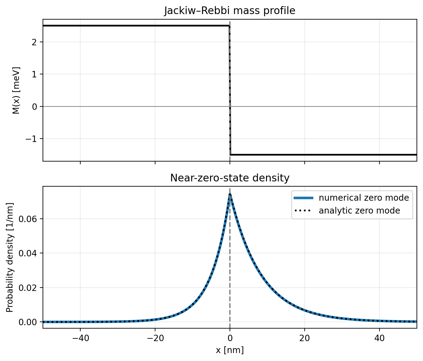
Fig. 23.13.1 Mass profile and numerical and analytic probability densities of the near-zero Jackiw–Rebbi state.

As expected, the bound state is localized at the interface where the mass term changes sign, and its numerical density overlaps with the analytic envelope from Eq. (23.2.6).

23.14. Full code

__copyright__ = "Copyright 2022-2026, Nanoacademic Technologies Inc."

import pathlib
import numpy as np
from numpy.typing import NDArray
from matplotlib import pyplot as plt
from qtcad.device import constants as ct
from qtcad.device import materials as mt
from qtcad.device.mesh1d import Mesh
from qtcad.device import Device
from qtcad.device.analysis import integrate
from qtcad.device.electron_kp import ElectronKPModel
from qtcad.device.electron_kp import ElectronKPParameter
from qtcad.device.pauli import sigma_vec
from qtcad.device.schrodinger import Solver
from qtcad.device.schrodinger import SolverParams

# File paths -----------------------------------------------------------------
script_dir = pathlib.Path(__file__).parent.resolve()
path_mesh = script_dir / "meshes" / "jackiw_rebbi_1d.msh"
path_out = script_dir / "output"
path_fig = path_out / "electron_kp_jackiw_rebbi.png"

# Model parameters -----------------------------------------------------------
# Units.
nm = 1e-9
meV = ct.e / 1000
# Mass-energy term.
mass_parameter_name = "jackiw_rebbi_mass"
M_L = 2.5 * meV
M_R = -1.5 * meV
# Velocity term.
hbar_v = 25.0 * meV * nm
# Plotting window.
plot_window = 50.0 * nm
# Number of states to solve the Schrödinger equation for.
num_states = 8

# Electron k · p model -------------------------------------------------------
def mass_term_sigma_z(mass: float) -> NDArray[np.float64]:
    """Convert a scalar mass into a Jackiw–Rebbi mass term.

    Args:
        mass: A scalar mass corresponding to M(x) at a given point in space.

    Returns:
        Matrix-valued coefficient mass * sigma_z representing the second term in the
        Jackiw-Rebbi Hamiltonian M(x) * sigma_z at a given point in space.
    """

    return mass * sigma_vec[2]

def build_jackiw_rebbi_model() -> ElectronKPModel:
    """Build the two-band Jackiw–Rebbi electron k·p model.

    The Hamiltonian is

        H = hbar v k_x sigma_x + M(x) sigma_z.

    The mass term M(x) is resolved from the region materials through an 
    ElectronKPParameter.
    The velocity term (proportional to sigma_x) is constant over all space.

    Returns:
        Electron k·p model describing the Jackiw–Rebbi model.
    """

    mass_term = ElectronKPParameter(
        mass_parameter_name, # Connect the model to material parameter.
        transform=mass_term_sigma_z, # Get mass term proportional to sigma_z.
    )

    velocity_term = hbar_v * sigma_vec[0] # Velocity term proportional to sigma_x.

    model = ElectronKPModel(
        bands=2,
        constant=mass_term,
        linear={"x": velocity_term},
    )

    return model

# Region materials -----------------------------------------------------------
def build_region_materials() -> tuple[mt.Material, mt.Material]:
    """Create materials carrying the electron k·p mass parameter.

    Returns:
        Materials representing the two different regions of the device.

        Both materials possess a k·p parameter, labelled `"jackiw_rebbi_mass"`, 
        which is set via `set_electron_kp_param`.
    """

    left_trivial = mt.Material({"name": "Left"})
    left_trivial.set_electron_kp_param(
        mass_parameter_name,
        M_L,
    )

    right_topological = mt.Material({"name": "Right"})
    right_topological.set_electron_kp_param(
        mass_parameter_name,
        M_R,
    )

    return left_trivial, right_topological

# Device setup ---------------------------------------------------------------
def build_device() -> Device:
    """Load the mesh, assign regions, and attach the electron k·p model.

    Returns:
        Device containing the Jackiw–Rebbi mesh, material regions, boundary
        conditions, and Jackiw–Rebbi k·p model.
    """

    # Create the materials.
    left_trivial, right_topological = build_region_materials()
    # Create the device.
    mesh = Mesh(nm, str(path_mesh))
    dvc = Device(mesh, conf_carriers="e")
    ## Set the regions.
    dvc.new_region("left_trivial", left_trivial)
    dvc.new_region("right_topological", right_topological)
    ## Set the boundary conditions.
    dvc.new_insulator("left_bnd")
    dvc.new_insulator("right_bnd")
    ## Set the k·p model.
    jackiw_rebbi_model = build_jackiw_rebbi_model()
    dvc.set_electron_kp_model(jackiw_rebbi_model)

    return dvc

# Schrodinger solve ----------------------------------------------------------
def solve_schrodinger(dvc: Device) -> None:
    """Solve the electron k·p Hamiltonian with the Schrödinger solver.

    Args:
        dvc: Device whose electron k·p Hamiltonian is to be solved.
    """

    params = SolverParams()
    params.num_states = num_states
    params.tol = 1e-10
    params.verbose = False

    solver = Solver(dvc, solver_params=params)
    solver.solve()

# Resolved mass profile ------------------------------------------------------
def mass_profile_from_model(dvc: Device) -> NDArray[np.float64]:
    """Return the resolved Jackiw–Rebbi mass profile on global mesh nodes.

    Args:
        dvc: Device with an attached Jackiw–Rebbi electron k·p model.

    Returns:
        Jackiw–Rebbi mass profile on global nodes of the mesh over which dvc is 
        defined.
    """

    # Get all coefficients resolved over the device.
    resolved = dvc.electron_kp_model.resolve_device_coefficients(dvc)
    # Get the constant term.
    constant_term = resolved.get_coefficients_for_pair(("1", "1"))
    # Convert to global nodes.
    constant_term_nodes = dvc.mesh.toglobal(constant_term[0])

    # Get the M(x) parameter.
    mass_term = 0.5 * (
        constant_term_nodes[..., 0, 0] - constant_term_nodes[..., 1, 1]
    )
    mass_term = np.real(mass_term)

    return mass_term

# Analytic bound state -------------------------------------------------------
def analytic_bound_state(
    mesh: Mesh,
) -> NDArray[np.complex128]:
    """Return the analytic Jackiw–Rebbi zero mode on global mesh nodes.

    Args:
        mesh: Mesh over which the analytic state is defined.

    Returns:
        Normalized two-component analytic bound-state wavefunction sampled on the
        mesh global nodes.
    """
    x = mesh.glob_nodes[:, 0]

    envelope = np.where(
        x < 0.0,
        np.exp(M_L * x / hbar_v),
        np.exp(M_R * x / hbar_v),
    )
    # The zero-energy mode is proportional to the sigma_y eigenstate.
    spinor = np.array([1.0, -1.0j], dtype=complex) / np.sqrt(2.0)
    wavefunction = envelope[:, np.newaxis] * spinor[np.newaxis, :]

    # Apply the analytic normalization factor.
    norm = np.sqrt(
        -2 * M_L * M_R
        / ((M_L - M_R) * hbar_v)
    )

    return wavefunction * norm

def band_weights_from_wavefunction(
    mesh: Mesh,
    wavefunction: NDArray[np.complex128],
) -> NDArray[np.float64]:
    """Integrate the band weights of a two-component wavefunction.

    Args:
        mesh: Mesh over which the wavefunction is defined.
        wavefunction: Two-component wavefunction sampled on the global nodes of mesh.

    Returns:
        Normalized probability weight carried by each band component.
    """

    component_densities = np.abs(wavefunction) ** 2
    weights = np.array(
        [
            integrate(mesh, component_densities[:, band_index])
            for band_index in range(component_densities.shape[-1])
        ],
    )

    return weights / np.sum(weights)

def relative_band_phase(
    mesh: Mesh,
    wavefunction: NDArray[np.complex128],
) -> float:
    """Return the relative phase between the two band components.

    Args:
        mesh: Mesh over which the wavefunction is defined.
        wavefunction: Two-component wavefunction sampled on the global nodes of mesh.

    Returns:
        Phase angle, in radians, of the integrated interband coherence.
    """

    coherence = integrate(mesh, np.conj(wavefunction[:, 0]) * wavefunction[:, 1])

    return np.angle(coherence)

# Plotting -------------------------------------------------------------------
def plot_near_zero_states(
    x: NDArray[np.float64],
    mass_profile: NDArray[np.float64],
    num_wavefunction: NDArray[np.complex128],
    an_wavefunction: NDArray[np.complex128],
) -> None:
    """Plot the mass profile and compare numerical and analytic densities.

    Args:
        x: Mesh-node coordinates sorted by increasing x coordinate.
        mass_profile: Jackiw–Rebbi mass profile sampled on the sorted nodes.
        num_wavefunctions: Multiband eigenfunctions sorted on the same nodes.
        an_wavefunction: Analytic bound-state wavefunction sampled on x.
    """

    # Get densities associated to wavefunctions.
    num_density = np.sum(np.abs(num_wavefunction) ** 2, axis=-1)
    analytic_density = np.sum(np.abs(an_wavefunction) ** 2, axis=-1)
    # Scale the positions.
    x_nm = x / nm

    # Create the figure.
    fig, axes = plt.subplots(2, 1, figsize=(7.0, 6.0), sharex=True)
    ## Mass profile plot.
    axes[0].plot(x_nm, mass_profile / meV, color="black", linewidth=2.0)
    axes[0].axhline(0.0, color="0.5", linewidth=0.8)
    axes[0].axvline(0.0, color="0.5", linestyle="--")
    axes[0].set_ylabel("M(x) [meV]")
    axes[0].set_title("Jackiw–Rebbi mass profile")
    axes[0].grid(alpha=0.25)

    ## Densities plot.
    num_style = {"linewidth": 3.0, "linestyle": "-"}
    axes[1].plot(
        x_nm,
        num_density * nm,
        label="numerical zero mode",
        **num_style,
    )
    an_style = {"linewidth": 2.0, "linestyle": ":", "color": "black"}
    axes[1].plot(
        x_nm,
        analytic_density * nm,
        label="analytic zero mode",
        **an_style
    )
    axes[1].axvline(0.0, color="0.5", linestyle="--")
    axes[1].set_xlabel("x [nm]")
    axes[1].set_ylabel("Probability density [1/nm]")
    axes[1].set_title("Near-zero-state density")
    axes[1].grid(alpha=0.25)
    axes[1].legend()
    axes[1].set_xlim(-plot_window / nm, plot_window / nm)

    fig.tight_layout()

    # Save the figure.
    path_out.mkdir(parents=True, exist_ok=True)
    fig.savefig(path_fig, dpi=200, bbox_inches="tight")
    plt.close(fig)

# Analysis -------------------------------------------------------------------
if __name__ == "__main__":

    # Create the device.
    dvc = build_device()
    # Solve the Schrödinger equation.
    solve_schrodinger(dvc)
    # Print the k·p model attached to the device.
    dvc.electron_kp_model.print()

    # Energies of the states.
    energies_mev = dvc.energies / meV
    # Find the near-zero energy state.
    near_zero_index = np.argsort(np.abs(energies_mev))[0]
    # Weight of the eigenstates projected onto each band.
    band_weights = dvc.band_weight()
    # Numerical bound state on global nodes.
    num_wavefunction = dvc.eigenfunctions[:, near_zero_index, :]
    # Compute the analytic bound state on the global nodes.
    an_wavefunction = analytic_bound_state(dvc.mesh)
    # Weight of the analytic wavefunction projected onto each band.
    analytic_band_weights = band_weights_from_wavefunction(
        dvc.mesh,
        an_wavefunction,
    )

    print(f"\nState {near_zero_index}")
    print("Energy [meV]:")
    print(energies_mev[near_zero_index])

    print("\nAnalytic comparison")
    print("Numerical band weights:")
    print(band_weights[near_zero_index])
    print("Analytic band weights:")
    print(analytic_band_weights)
    print("Numerical relative phase [rad]:")
    print(relative_band_phase(dvc.mesh, num_wavefunction))
    print("Analytic relative phase [rad]:")
    print(relative_band_phase(dvc.mesh, an_wavefunction))

    # Post-process data for visualization.
    ## Order the global nodes.
    order = np.argsort(dvc.mesh.glob_nodes[:, 0], kind="stable")
    x = dvc.mesh.glob_nodes[order, 0]
    ## Order the wavefunctions
    num_wavefunction = num_wavefunction[order, :]
    an_wavefunction = an_wavefunction[order, :]
    # Order the mass, M(x).
    mass_profile = mass_profile_from_model(dvc)
    mass_profile = mass_profile[order]

    plot_near_zero_states(
        x,
        mass_profile,
        num_wavefunction,
        an_wavefunction,
    )